JAX is a Python library offering high performance in machine learning with XLA and Just In Time (JIT) compilation. Its API is similar to NumPy’s with a few differences. JAX ships with functionalities that aim to improve and increase speed in machine learning research. These functionalities include:

• Automatic differentiation
• Vectorization
• JIT compilation

Flax is a neural network library for JAX. This article will cover how to track JAX and Flax models with Comet.

Let’s get started.

Getting started

Start by installing Comet.

pip install comet_ml

Next, install JAX and Flax.

pip install -q jax jaxlib flax

Import the libraries you’ll use in this project.

import comet_ml
import jax
import jax.numpy as jnp                # JAX NumPy

from flax import linen as nn           # The Linen API
from flax.training import train_state  # Useful dataclass to keep train state

import numpy as np                     # Ordinary NumPy
import optax                           # Optimizers
import tensorflow_datasets as tfds     # TFDS for MNIST

Log parameters

In this project, you’ll build a simple Convolutional Neural Network using the MNIST dataset. Define the network parameters and log them to Comet.

To achieve that, create a Comet experiment.

experiment = comet_ml.Experiment(
    api_key="YOUR_API_KEY",
    project_name="JAX_Flax_CNN", log_code=True)

Next, use this experiment to log the network metrics.

# these will all get logged
params = {
    "features_1": 32,
    "kernel_size": 3,
    "window_shape": 2,
    "categories": 10,
    "features_2": 64,
    "features_3":256,
    "strides": 2,
    "cross_entropy_loss": "softmax_cross_entropy",
    "dataset": "MNIST"
}

experiment.log_parameters(params)

Flax network definition

In Flax, networks are defined using the Linen package. Define a simple CNN network using the parameters defined above.

Flax networks are defined explicitly using setup or inline using nn.compact.

setup vs compact

class CNN(nn.Module):
  """A simple CNN model."""

  @nn.compact
  def __call__(self, x):
    x = nn.Conv(features=params['features_1'], kernel_size=(params['kernel_size'], params['kernel_size']))(x)
    x = nn.relu(x)
    x = nn.avg_pool(x, window_shape=(params['window_shape'], params['window_shape']), strides=(params['strides'], params['strides']))
    x = nn.Conv(features=params['features_2'], kernel_size=(params['kernel_size'], params['kernel_size']))(x)
    x = nn.relu(x)
    x = nn.avg_pool(x, window_shape=(params['window_shape'], params['window_shape']), strides=(params['strides'], params['strides']))
    x = x.reshape((x.shape[0], -1))  # flatten
    x = nn.Dense(features=params['features_3'])(x)
    x = nn.relu(x)
    x = nn.Dense(features=params['categories'])(x)
    return x

Compute metrics

Next, define the metrics used to compute loss and accuracy during training. In JAX, we compute the loss using the Optax library.

def cross_entropy_loss(*, logits, labels):
  labels_onehot = jax.nn.one_hot(labels, num_classes=params['categories'])
  return optax.softmax_cross_entropy(logits=logits, labels=labels_onehot).mean()

The compute_metrics function will calculate and return the loss and accuracy.

def compute_metrics(*, logits, labels):
  loss = cross_entropy_loss(logits=logits, labels=labels)
  accuracy = jnp.mean(jnp.argmax(logits, -1) == labels)
  metrics = {
      'loss': loss,
      'accuracy': accuracy,
  }
  return metrics

Loading data in JAX

JAX and Flax don’t ship with data loaders. Therefore, you have to use data loaders from TensorFlow and PyTorch.

In this case, we load the dataset using TensorFlow.

def get_datasets():
  """Load MNIST train and test datasets into memory."""
  ds_builder = tfds.builder('mnist')
  ds_builder.download_and_prepare()
  train_ds = tfds.as_numpy(ds_builder.as_dataset(split='train', batch_size=-1))
  test_ds = tfds.as_numpy(ds_builder.as_dataset(split='test', batch_size=-1))
  train_ds['image'] = jnp.float32(train_ds['image']) / 255.
  test_ds['image'] = jnp.float32(test_ds['image']) / 255.
  return train_ds, test_ds

Create Flax training state

In Flax, we create a training state to store all the training information, such as parameters and the optimizer state. This is achieved using train_state from Flax. In the training state function:

• Create an instance of the network.
• Call the init method to obtain network parameters by passing a sample data point.
• Return the training state by applying the model while passing the parameters and the optimizer.

def create_train_state(rng, learning_rate, momentum):
  """Creates initial `TrainState`."""
  cnn = CNN()
  params = cnn.init(rng, jnp.ones([1, 28, 28, 1]))['params']
  tx = optax.sgd(learning_rate, momentum)
  return train_state.TrainState.create(
      apply_fn=cnn.apply, params=params, tx=tx)

Network training

The next step is to define the model training functions. Let’s start by defining a function that will train the network for one step.

The function:

• Applies the network to a batch of data and computes the loss and logits.
• Computes gradients with respect to the loss.
• Applies the gradients to obtain a new state.
• Computes and returns the model metrics.

Applying jax.jit makes the function run faster.

@jax.jit
def train_step(state, batch):
  """Train for a single step."""
  def loss_fn(params):
    logits = CNN().apply({'params': params}, batch['image'])
    loss = cross_entropy_loss(logits=logits, labels=batch['label'])
    return loss, logits
  grad_fn = jax.value_and_grad(loss_fn, has_aux=True)
  (_, logits), grads = grad_fn(state.params)
  state = state.apply_gradients(grads=grads)
  metrics = compute_metrics(logits=logits, labels=batch['label'])
  return state, metrics

Next, define a training function that applies the above training step. The function:

• Shuffles the training data.
• Runs the training step for each batch.
• Obtains the training metrics from the device using jax.device_get
• Computes the mean of the metrics from each batch.
• Returns the new state together with the model metrics.

def train_epoch(state, train_ds, batch_size, epoch, rng):
  """Train for a single epoch."""
  train_ds_size = len(train_ds['image'])
  steps_per_epoch = train_ds_size // batch_size

  perms = jax.random.permutation(rng, train_ds_size)
  perms = perms[:steps_per_epoch * batch_size]  # skip incomplete batch
  perms = perms.reshape((steps_per_epoch, batch_size))
  batch_metrics = []
  for perm in perms:
    batch = {k: v[perm, ...] for k, v in train_ds.items()}
    state, metrics = train_step(state, batch)
    batch_metrics.append(metrics)

  # compute mean of metrics across each batch in epoch.
  batch_metrics_np = jax.device_get(batch_metrics)
  epoch_metrics_np = {
      k: np.mean([metrics[k] for metrics in batch_metrics_np])
      for k in batch_metrics_np[0]}



  return state, epoch_metrics_np['loss'],epoch_metrics_np['accuracy'] * 100

Network evaluation

The evaluation step checks the performance of the network on the testing data.

@jax.jit
def eval_step(params, batch):
  logits = CNN().apply({'params': params}, batch['image'])
  return compute_metrics(logits=logits, labels=batch['label'])

Next, define a function that applies the evaluation step to the testing data. The function also obtains the evaluation metrics from the device.

def eval_model(params, test_ds):
  metrics = eval_step(params, test_ds)
  metrics = jax.device_get(metrics)
  summary = jax.tree_util.tree_map(lambda x: x.item(), metrics)
  return summary['loss'], summary['accuracy']

Want to try Comet for yourself? Sign up for a free account today!

Train the Flax network

You now have all the required building blocks for training the Flax CNN.

Download data

Start by downloading the data.

train_ds, test_ds = get_datasets()

Set random seed

JAX requires pure functions. This means that they should not have any side effects. Therefore, even the random seed generation should be reproducible. These numbers are generated using jax.random.PRNGKey.

rng = jax.random.PRNGKey(0)
rng, init_rng = jax.random.split(rng)

Initialize train state

Create a training state using the function defined earlier.

learning_rate = 0.1
momentum = 0.9

state = create_train_state(init_rng, learning_rate, momentum)
del init_rng  # Must not be used anymore.

Log model metrics

The next step is to apply the training function for the desired number of epochs. At each epoch, we:

• Obtain the training and test metrics.
• Log the metric to Comet.
• Print the metrics to the console.

num_epochs = 10
batch_size = 32

training_loss = []
training_accuracy = []
testing_loss = []
testing_accuracy = []


for epoch in range(1, num_epochs + 1):
  # Use a separate PRNG key to permute image data during shuffling
  rng, input_rng = jax.random.split(rng)
  # Run an optimization step over a training batch
  state, train_loss, train_accuracy = train_epoch(state, train_ds, batch_size, epoch, input_rng)
  training_loss.append(train_loss)
  training_accuracy.append(train_accuracy)
  # Evaluate on the test set after each training epoch 
  test_loss, test_accuracy = eval_model(state.params, test_ds)
  testing_loss.append(test_loss)
  testing_accuracy.append(test_accuracy)

  experiment.log_metric("train_loss", train_loss, step=None, epoch=epoch, include_context=True)
  experiment.log_metric("train_accuracy", train_accuracy, step=None, epoch=epoch, include_context=True)
  experiment.log_metric("test_loss", test_loss, step=None, epoch=epoch, include_context=True)
  experiment.log_metric("test_accuracy", test_accuracy, step=None, epoch=epoch, include_context=True)
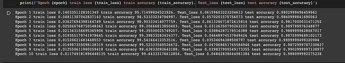
  print(f'Epoch {epoch} train loss {train_loss} train accuracy {train_accuracy}. Test_loss {test_loss} test accuracy {test_accuracy}')

Log model charts

Since the metrics are saved in a list, you can plot the data and log the chart to Comet.

fig = plt.figure(figsize=(8, 6))

plt.plot(training_loss, label="Training")
plt.plot(testing_loss, label="Test")
plt.xlabel("Epoch")
plt.ylabel("Accuracy")
plt.legend()
plt.show()

experiment.log_figure(figure_name="Loss visualization", figure=fig)

Don’t forget to end the experiment once you are done

experiment.end()

View the experiment on Comet

Click the link generated when you end the experiment to view the experiment on Comet’s UI.

The Charts dashboard shows plots of the metrics you logged.

The hyperparameters dashboard shows the logged parameters.

The Graphics dashboard shows all the logged charts.

Final thoughts

In this article, you have seen how to track Flax experiments with Comet. Apart from that, you have also seen how to:

• Load datasets in JAX.
• Define networks with Flax.
• Create a training state in Flax.
• Train CNN in Flax.

Resources

• Notebook
• JAX
• Flax