Stanford Research Series: Grand Digital Piano: Multimodal Transfer of Learning of Sound and Touch
Authors: Ernesto Evgeniy Sanches Shayda (esanches@stanford.edu), Ilkyu Lee (lqlee@stanford.edu)
I. MOTIVATION
Musical instruments have evolved during thousands of years allowing performers to produce almost all imaginable musical sounds of various timbre, pitch, loudness and duration. Speaking about keyboard instruments, the current grand piano mechanism is the result of a series of inventions and improvements and is a very complex mechanical system. During past decades a new area of research about creating digital instruments that have same feel and sound as original acoustic instruments have gained popularity [1]. There was a partial success in developing a digital piano with realistic sound and touch: most devices recreate basic properties of sound, however it can be noticed that the models are far from perfection due to the following reasons.
Most digital pianos use sample-based synthesis, meaning that for every piano key a finite number of ”sample tones” of a real acoustic instrument are recorded, and then the resulting sound when a key is pressed is just one of the samples or a combination of the samples. As a result, an infinite variety of timbres of a real instrument is reduced to just a few, corresponding to number of samples per key that are prerecorded.
There are also pianos that use mathematical models of the acoustic instrument to produce sounds without use of ”sample tones” [2]. Theoretically this allows to recreate an infinite variety of sounds of the original instrument. However, the models require a lot of assumptions about internal physics of piano action mechanism and about the sound production process and use hand-designed parts, which are not guaranteed to be equivalent to the mechanics of a real instrument.
We are going to improve the methods described above, using machine learning to train a physically-based model of piano, which will allow to produce new, previously unheard sounds during the training, depending on how performer plays the instrument.
II. PRIOR WORK
Generating realistic sound data in a form of exact waveforms, without usage of hand-crafted aggregate sound features (such as spectrograms or mel frequency cepstral coefficients) was made possible by a line of research started from WaveNet model [3]. Recently a very detailed NSynth dataset [4] of notes played on different musical instruments was collected, which make possible to use models such as WaveNet to generate realistic musical instruments sound. An improved model for musical sounds generation was recently proposed [5], utilizing generative adversarial networks to make generated sounds even closer to real ones.
While sound generation algorithms significantly advanced during past years, there is a difficulty in using the proposed algorithms in actual digital instruments, because the mentioned algorithms are concerned only with one aspect: generating realistic sound. However very noticeable part of playing an instrument is a connection between performer’s actions and the actual sound that is generated. While existing models support simple conditioning, allowing to generate sounds of varying loudness and timbre, exact connection between physical actions by a performer and the resulting sound was not studied in context of artificial intelligence models of sound generation.
In this work we are going to close this gap by introducing a multi-modal model, that analyzes performer’s actions and resulting sound jointly, allowing to generate appropriate sound based on the way how performer plays the instrument. Additionally, we develop a transfer of learning method, that allows to learn the model once on very precise equipment and high quality acoustic instruments, and then apply the resulting model on different variants of target instruments of different price and quality, aiming at obtaining closest possible sound and feel to the original instrument in all cases. While the methods can be applied to any musical instrument, where performer’s actions and resulting sound can be captured, in this work we focus on creating a realistic digital piano, which is one of the most used digital instruments.
III. PROBLEM FORMULATION
We consider multiple modalities, that are always present in a musical performance. We start from ”touch” — a way how performer plays, and ”sound” — the resulting music that is heard. Each modality can be represented as a time series containing information about what is happening at each moment of time. For piano, ”touch” modality consists of a physical state of all keys, namely positions or velocities as a function of time. Additionally, other controls can be recorded as well, such as positions or velocities of piano pedals.
Considering just these two modalities, it is possible to make a generative model, as long as there is a possibility to do the following:
- Precisely record touch and sound during the training phase on a reference instrument.
- Precisely record touch during the performance or a testing phase.
- Ensure that meaning of recorded touch (that can be described by an expected sound to be heard from such touch) on a reference instrument, and on performance instrument, are same.
We notice that there is a number of difficulties arising in this setting:
- First, for recording data from real instrument, we want to apply non-invasive measurement, to prevent destruction or degradation of the instruments while conducting research. This means, that we are not going to modify the acoustic instrument and record data from the inside, or attach arbitrary devices to the instrument using adhesives or use other possibly irreversible techniques.
- There are multiple ways to measure touch using sensors, that can be grouped into contact-based and non-contact methods. According to the previously stated requirements, for collecting training data on real instrument we are going to use non-contact methods. Most efficient method in this group is laser distance sensing [6]. The method is very precise, but is usable only in laboratory conditions: arbitrary hand movements can block laser light and interfere with measurements. As a conclusion, we are going to use laser distance measurement, but only for collecting training data for ”touch” modality.
- For the testing or a performance phase, we want to apply robust method for measuring the data, to prevent giving special instructions to the performers, and just let them use the instrument as they normally would. This prevents usage of non-contact measurement techniques from outside of the instrument. Because of that, for the test phase, we consider a possibility to apply contact-based methods of measurement and also to apply modifications to the digital instruments for easier measurement.
This considerations show that there will be a problem of difference in ”touch” data in training and testing phases, requiring a use of Transfer of Learning methods. We propose a solution of this problem by adding new modalities: Instead of creating a model ”Touch → Sound”, we will create a conditional model ”Touch → Intermediate modality 1 → Intermediate modality 2 → … → Sound”. Either touch, or one of the intermediate modalities may not be available during a training or testing phases — in this case we will train auxiliary models to fill in missing modalities; and after filling in the missing data we will be able to do complete transfer of learning from the input in training stage to whatever input will be available in the testing stage, allowing to produce equivalent sounds.

IV. PRACTICAL IMPLEMENTATION
We consider the following input time series that are possible to record either in training or testing or in both phases:
- Laser distance sensor data. It is possible to record such data both for source (acoustic) and for target (digital instrument). However during testing phase the data will not be available for digital instrument. We are evaluating two sensors for touch modeling:
- Semiconductor miniature laser distance sensor VL53L0X. It has default sampling rate of 33 measurements per second and deviation of measurements around 2% of the measured value. There is also an updated version named VL53L1X, that allows up to 50Hz sampling rate.
- Simple LIDAR: RPLIDAR A1M8, which can be used as a fixed position laser distance sensor as well by manually disabling rotation of the sensor head. It has sampling rate of 2 thousands measurements per second and deviation of measured value of 1%.
- Accelerometer and gyroscope sensor: miniature sensors can be attached to piano keys of digital piano and measure the positions with rate of up to 1000 measurements per second.
- Hall effect magnetic sensors: such miniature sensors can also be attached to digital piano keys, allowing to measure distance to a magnet, that needs to be attached to digital piano case.
- Ambient light proximity sensors: such sensors provide non-contact measurement of small distance below 10 millimeters. In contrast to laser sensors, such sensors have lower cost and can be mounted inside the digital piano for measuring distance to each key.
- MIDI sensors (recording approximate key velocity at the moment of piano key strike), that are already present in most digital piano instruments. This allows to have a reference sensor data. However, MIDI sensors do not record data continuously, they integrate the data and just provide a single velocity measurement for each key press, therefore they do not allow to precisely model the touch.
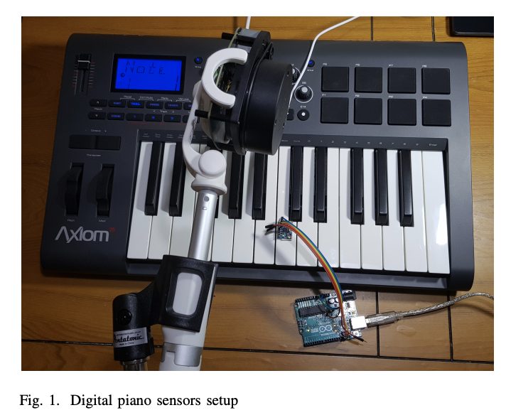
We have compared two measurement solutions for use with acoustic piano in Table I. Because grand piano measurements are done only once and can be reused on multiple digital devices, it is beneficial to use highest precision equipment for this part of work. Therefore we continue the remaining experiments using the RPLidar A1M8 distance sensor. For the intermediate modality we choose to narrow our selection to the Accelerometer and MIDI sensors for the following reason: MIDI sensors are present in almost all digital pianos that have MIDI output and can be used without adding external hardware; and Accelerometer sensors usually have built-in gyroscope, which allows to capture angular velocity, which is the exact mechanical parameter that is required to model dynamics of the key. In contrast, light and magnetic sensors only indirectly measure the mechanics: there is a nonlinear relationship between angular position and velocity, and resulting measurement of magnetic field and light intensity. The final arrangement of sensors for modeling a single piano key is shown on Figure 1, consisting of a Lidar that is also used with grand piano, an accelerometer, attached to a key, and internal MIDI sensors of a digital keyboard.
V. TRANSFER OF LEARNING MODELS
The physical setup, described in previous section, shows a need to model the following sequence of dependencies:
Laser sensor data (available on digital and acoustic piano during training; not available during testing) → {Accelerometer, MIDI sensor data} (available only on digital piano during training and testing) → Sound (available only on real piano during training and testing; must be re-created on digital piano)
While ideally we would generate sound from laser sensor data during performance, this most precise method of measurement is not available at the testing stage. Therefore we first transform Laser sensor data into a corresponding (predicted) data from other sensors, that will be available in the testing stage. This sensor data is available only on digital piano, because it involves contact measurement. At the same time, real sound data is available only on acoustic piano. This dictates a need to create two big datasets and to train two classes of machine learning models:
- On Digital piano: take ”Laser sensor data” as an input and predict ”Other sensors data, including MIDI, accelerometer”
- After having such model, apply it on Acoustic piano, by predicting other sensor data, which is unavailable on Acoustic piano.
- On Acoustic piano, take predicted other sensor data as an input, and train a machine learning model to predict sound from it.
- Apply this model on digital piano to generate realistic sound from other sensors, present only on digital piano.
The overall dataset will be highly multi-modal, containing at least two main time series (Laser sensor data, resulting sound) and many auxiliary time series (intermediate sensors, present only on digital piano).
VI. MACHINE LEARNING MODELS
A. Sound models
We start from examining the largest part of the data: musical instruments sound. We have recorded sound of two notes (middle C and G keys) from digital and acoustic piano, trying to record as many as possible different ways of touching the piano keys. This resulted in initial dataset, that can be further extended to an octave (8–13 keys) or full piano range (88 keys). In the following two sections we conduct experiments on the sound data only for initial analysis and understanding of the data.
B. Supervised classification between digital and acoustic instrument
We considered a task of predicting whether the note sounded is from acoustic or digital piano. We used raw representation of 2 seconds of sound, which were recordings of C4 and G4 notes on both a grand piano and a Yamaha YDP-141 digital piano, and pre-processed the recordings to normalize audio and trim silence. There were 132 recordings in total, and with a sampling rate of 44100 Hz, allowing for a total feature space of 132 samples of dimension 2*44100.
Then, applying a binary labelling system for digital and acoustic, we utilized a multi-layer perceptron (MLP) neural network with a hidden layer of 100 units and ReLU as the activation function for classification. Given a 80–20 training testing split, the resulting testing accuracy was 81%. This gives confidence in the ability of models to differentiate acoustic and digital sounds, allowing for further data analysis.
C. Unsupervised learning of sound representation
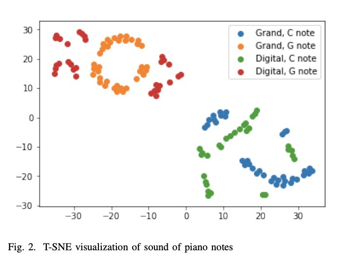
We have applied T-SNE algorithm [7] on a collected initial dataset of two notes on two instruments (Figure 2). Learned representation indeed shows that digital and acoustic instruments are different and separable in the latent space, and also that different notes have distinguishable characteristics. This initial results show that the big task of this project is also feasible, and we are going to proceed with collecting the remaining sensors data and training the main models for sound generation.
D. Feed-forward neural network vs. regression model for intermediate modality prediction
We start the actual task of transforming acoustic piano touch data into a common format from modeling of Laser MIDI sensor relationship using an MLP neural network and a regression model. Firstly, on the digital piano, the C4 and G4 notes were pressed with varying force and hence key velocity, with the laser sensor measuring the displacement of the key with time. The corresponding MIDI data of the key velocity was also recorded with time and then normalized by dividing by 127 (only for regression model, as we want to keep the discrete values for MLP multinomial classification).
Then, after combining the C and G data, the 1-D time series data for both the laser position and MIDI velocity were reshaped into 2-D arrays, wherein each row represented 20 milliseconds of data, with a shift of 10 millisecond from the first entry of a row and the first entry of the next row. The resulting feature space was further processed to remove any portions wherein the MIDI value does not change given a 20 millisecond frame, as prediction is impossible otherwise. Finally, the last value of the MIDI velocity per row was used as output space, such that the prediction is going from L(t−n : t) → M(t), where L(t) and M(t) are the Laser and MIDI data, respectively, with n representing 20 milliseconds (882 features).
The dataset was then fed into two models: an MLP neural network with a single hidden layer of 100 units and a simple ridge regression model with mean squared error loss. We would expect the ridge regression model to perform better than MLP, since given a true label (velocity), the multinomial softmax loss of MLP would penalize wrong classification of velocity regardless of how close the predicted velocity is to the true one. On the other hand, a regression model not only allows for prediction of velocity values that may be absent in the training data but also penalizes a prediction closer to the true value much less than a prediction that is further away.
As expected, the MLP network gave a testing accuracy of 45%, while the ridge regression gave an error of 26%. Even though the regression model performs better, its error is too high; we then proceed with a recurrent neural network (RNN) to go about the prediction of MIDI given laser data.
E. Recurrent network for intermediate modality prediction
Unlike feed-forward networks, RNNs contain a feedback loop that takes in a previous output yt−1 at time t − 1 as input at time t along with some original input xt. In this manner, one can think of RNNs as having memory, wherein sequential information is utilized to understand correlations in time-dependent events to aid in better prediction. Moreover, RNNs have the ability to do many-to-many prediction, which is desired here as we are predicting a full time series.
In our case, we use an RNN model with two stacked long short-term memory (LSTM) layers with 10 neurons in each layer, with mean squared error loss and rmsprop as the optimizer. Rather than doing a shifting window separation of data as the feature space, we simply divide the data into 2- second lengths, giving us 128 input vectors. In addition, in order to preserve the sequential nature of the predictions, we do not split our training and testing data randomly. In this manner, the loss was able to converge to about 0.086 with only a few epochs (4–6).
However, we notice that RNN cannot exactly predict such rapidly changing signal as a square wave in MIDI, which is difficult to approximate by a smooth function. We start from dividing the problem into two parts: predicting where MIDI events start, and predicting the actual value of MIDI event.
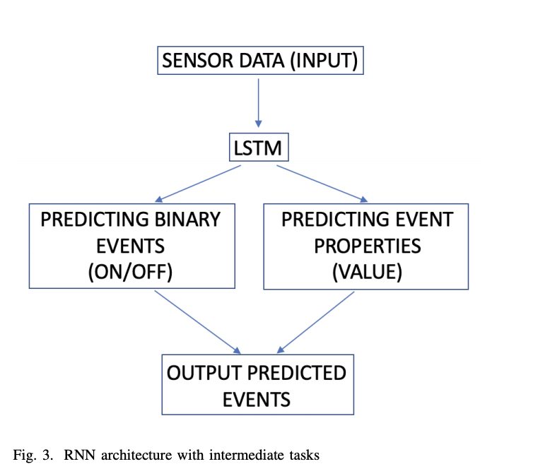
Therefore, we have implemented an architecture from Figure 3 to provide additional supervision to the network. The network still has an LSTM layer or multiple LSTM layers, that are then connected to two separate output layers: ”binary events” prediction layer has a sigmoid activation function to output probability of a fact that an event is currently happening. This layer is trained using cross-entropy loss to maximize likelihood of correctly predicting event start times. And ”event properties” layer has a linear activation and is trained with mean squared error loss, to minimize deviations in predicted event properties. Then two outputs are manually combined in a post-processing layer to output ”event properties” only if the binary model has predicted that there is an event currently. Such separation of the task into two subtasks allows to achieve faster convergence.
In figure 4 we present the resulting time series generated by the model. The model is able to correctly time the events, but still has difficulties in producing exact values, that we are going to solve by smoothing in the following section
F. Kalman filter for features extraction
Despite all information being available in the raw data, in previous sections we have seen number of difficulties in training neural networks. To aid the networks in solving the final task, we will incorporate a prior knowledge about basic physical model of a piano key. Piano key is a system with only one degree of freedom, and can be fully characterized by angular position of a key. Further, we can compute respective velocity and acceleration to model dynamic behavior. Because sensors provide noisy data, and also do not provide all three parameters simultaneously, we can use Kalman filter [8] to obtain reliable estimation of
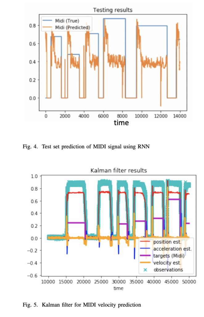
key dynamics. This will transform a single raw feature — position, into three smoothed features — position, velocity and acceleration.
We notice that velocity modeled by Kalman filter (Figure 5) allows to predict MIDI values at the start of MIDI events just by a linear transformation (which is expected, because both sensors now measure velocity), allowing the system to operate without referring to RNN, or just using the RNN to correct possible non-linearities.
We further notice that we have more advanced sensor system now, compared to a simple Synthesizer Midi sensors. Therefore, one of the reasons of getting low accuracy of predicting Midi signal may be the fact that ground truth is far from perfection. Particularly, there is a subjective difference in what key velocity actually means on the digital and acoustic piano. Performing a subjective test measuring Mean Opinion Scores comparing different ways of interpreting velocity should answer the question whether Digital piano’s MIDI sensors can be used as a reference.
VII. SOUND GENERATION
While the full implementation of the described ideas require two models: for touch, described in previous sections, and for sound, in this work we will use an existing model for sound generation, conditioned on the predicted touch data. We use the TensorFlow implementation of WaveNet [9] and train initially on the acoustic piano recordings of G4 and C4.
The model generates a new sample at time t by maximizing the log-likelihood of a joint probability distribution of the data stream up to time t − 1. This is done by a product of conditional distributions of each element in the above time range, employed as softmax distribution after treating the data values with Mu-law commanding for preserving sound dynamic range and at the same time decreasing required bits per sample to 8 bits.
In this implementation, the model has 9 hidden dilated convolutional layers, with the dilation increasing by a factor of 2 as one progresses in the layers, allowing for exponential receptive field growth with depth. Given 1200 steps, the training loss (cross entropy between the output for each timestep) was reduced from 5.677 to 1.1. We note that the loss can be reduced even greater with more time, and there exists other implementations for parallelization that have not been tested at the time of writing.
In terms of actual audio generation, conditioning on the note can be done manually via differentiation in the original data name itself; however, we have not yet been able to successfully condition on the MIDI velocity. This serves as a good direction for future work to improve upon the sound generation with conditioning included.
VIII. EVALUATION AND CONCLUSIONS
We have done objective evaluation by computing loss values on the hold-out testing set, with the results presented in the corresponding sections. Kalman filter showed a good performance in conjunction with RNN for intermediate modality prediction. And Wavenets provided initial results on sound generation which should be improved however for generating realistic sound
Subjectively, the system is in the initial stage of showing results, that can be used by musicians. We believe that presented idea is novel and practically useful, and there is definitively an additional work required to make the models applicable on production devices.
Source code of this work and collected datasets are available at https://github.com/ernestosanches/AIPiano
IX. ACKNOWLEDGEMENTS
We would like to thank Anand Avati from Stanford University for helpful discussions regarding transfer of learning, and Professor Elena Abalyan from University of Suwon for guidance on musical aspects of the work.
X. CONTRIBUTIONS
- Ernesto Evgeniy Sanches Shayda — idea, data collection, supervised modeling of touch data.
- Ilkyu Lee — initial data analysis and sound generation modeling
