Stanford Research Series: Exploring Model Architectures and View-Specific Models for Chest Radiograph Diagnoses
Authors: Danny Takeuchi (dtakeuch@stanford.edu), Raymond Thai (raythai@stanford.edu), Kevin Tran (ktran23@stanford.edu)
This project tackles several current issues with automated chest X-ray radiography, specifically regarding work on the Stanford Irvin et al. CheXpert dataset. We have created one of the most comprehensive open-sourced X-ray classification models. Our model explores two aspects of X-ray classification: the significance of view-specific model training and the exploration of different model architecture. Using a featurized DenseNet with a Decision Tree, we ultimately achieved a new state-of-the-art accuracy of 0.93, surpassing Irvin et al.’s single model accuracy of 0.76 (accuracy of 0.907 when ensembled). However, we saw poor results when using view-specific models. We attribute these lackluster results to similarities in X-ray scans between view types and a lack of training data.
1 Introduction
Chest radiography is an imaging technique used in the screening, diagnosis, and management of many life threatening diseases. Automated chest radiograph interpretation at the level of practicing radiologists can improve workflow in many medical settings including clinical decision support and global health initiatives.
After discussing with Irvin et al, a Stanford machine learning group that compiled and analyzed CheXpert, we saw several potential areas of improvement. First, previous approaches to automating radiograph interpretation utilized a single model across various view-types (posteroanterior(PA), anteroposterior(AP), and lateral views). If more than one view is available for a particular patient, the models would output the maximum probability of the observations across the views. However, a shortcoming of these approaches is that the visibility and the appearance of certain diseases differs based on view type. For example, an enlarged cardiomediastinum is much more visible from a frontal view than a side or back view and it looks different depending on the view. Second, previous approaches did not conduct much research into optimal model architectures for diagnoses. Finally, prior work including that of the Stanford Machine Learning group, are closed source and not available to the public.
Our group aims to improve upon previous work and open-source our work to provide insight for future chest radiography research. First, we re implemented and open-sourced the approach of Irvin et al. Then, to investigate the significance of view type on final diagnoses, our group implemented view-specific models as opposed to having just a single model to classify all view view-types. These models were both trained and tested on X-ray scans of only one specific view type. Lastly, we implemented VGG19 and VGG16 convolutional neural networks, kernelized SVMs and a decision tree to compare the performance of these models with the baseline DenseNet121 that Irvin used.
Our group aims to improve upon previous work and open-source our work to provide insight for future chest radiography research. First, we re implemented and open-sourced the approach of Irvin et al. Then, to investigate the significance of view type on final diagnoses, our group implemented view-specific models as opposed to having just a single model to classify all view view-types. These models were both trained and tested on X-ray scans of only one specific view type. Lastly, we implemented VGG19 and VGG16 convolutional neural networks, kernelized SVMs and a decision tree to compare the performance of these models with the baseline DenseNet121 that Irvin used.
2 Recent Work
Irvin et al. created the CheXpert dataset of 224,316 chest radiographs. After experimenting with several residual neural networks, the group used DenseNet121 in order to label the presence of 14 radiographic chest observations. This is a state of the art approach that also uses different uncertainty policies. However, this group only uses one generic model for the three view types instead of assigning the classification task to the best performing model. The model also has the downside of having largely uninterpretable features. In Saad, Mohd Nizam et al.’s research, an SVM kernel achieved state-of-the-art results for classifying chest x-rays based on nodule location in lung zones.
Nair, Aditya, et al. creates three modified VGG models and attempts to ensemble them in order to produce accurate results on the CheXpert dataset. One model used a weighted Bagging classifier to give higher weightage to higher performing classifiers. Nair’s VGG models were a promising fit for radiograph classification because its deeper features are helpful for feature extraction. However, he only attempts to identify the presence of five diseases, instead of all 14 diseases. His results on those five were inconclusive. Bar, Yaniv, et al. uses the Decaf pre-trained CNN model to classify chest radiographs and also fails to account for the varying view types.
Zhang et al. attempts to interpret CNNs through decision trees to quantitatively analyze the rational of each CNN prediction. This greatly increased the interpretability of their results compared to only using CNN. We hope to build upon this work and use featurized CNNs with various SVMs and a decision trees. In doing so, we hope to have both more accurate results and more interpretable results.
3 Dataset
We used Irvin et al.’s CheXpert dataset to train our view-specific models. CheXpert is a large dataset of 224,316 chest X-rays of 65,240 patients with radiologist-labeled interpretations. Each individual X-ray scan belongs to a specific study for a specific patient ID. The study number represents a particular visit for each patient. We group predictions by both patient ID and study.
Each individual X-ray radiograph is represented by the image and a feature vector containing patient id, sex, age, study number, X-ray view-type, and a vector of fourteen expert-labeled observations. We clean the data to omit the sex and age features from the equation because we evaluate solely on the image and view-type.
We chose the CheXpert dataset because its ground truth labels are determined by a panel of experts and because we can leverage insights
from previous experiments that have utilized the dataset. For our models, we down-scaled and cropped the data into 224 x 224 images. Each image was then converted to an RGB tensor. Before processing each batch of images, we flattened them into a tensor of shape (batch-size, 3*224*224) or (batch-size, 150528). The dataset includes X-rays of the various view-types (posteroanterior, anteroposterior and lateral) which are distributed with a 13:72:15 ratio. We split our data for each view type into a training set, validation set, and test set with a ratio of 98:1:1.
4 Approach
First, we re-implemented Irvin et al’s approach to classifying X-rays for each patient with a DenseNet121. We worked off the open-source github repository of a healthcare analytics company. The repository partially implemented Irvin et al’s method by making predictions on individual scans with a DenseNet121.
We re-implemented the architecture of this model to incorporate patient and study information. By comparing our updated model to the original Github repository, we were able to quantify the benefits of classifying by patient as opposed to classifying by individual X-ray. We observed a 0.0254 increase in AUROC when evaluating the DenseNet121 on patients instead of on individual scans. The input to our model is a batch of 64 chest X-rays and the output is a batch of 64 14-bit vectors where each bit corresponds to the presence of a medical condition. To deal with uncertainty, we used the ones policy discussed in Irvin’s paper.
After re-implementing Irvin’s study, we attempted to build upon these results in two main ways. First, we tested our hypothesis that incorporating view type into classification would improve accuracy. We did this by training view-specific models and building a view specific classifier that would feed a given X-ray image into the appropriate view-specific model. Second, we implemented multiple new classification models in an attempt to improve upon the DenseNet121 baseline.
5 Methods — Incorporating View Type in Predictions
5.1 View Classifier
Our view classifier takes in an image as input and returns one of three views, frontal postero-anterior (PA), frontal antero-posterior (AP),
or lateral as an output. We built a view classifier because our system will need to determine the view of every X-ray scan to handle new
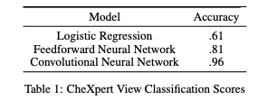
images and new datasets. The results for our view classifier are shown in Table 1 below.

Our baseline was multinomial logistic regression which used a linear layer and softmax because of its simplicity.
We then implemented a feed forward neural network, which we expected to outperform the baseline multinomial classifier because it could better abstract out high-level features. The input was run through two hidden Linear layers of size 150 and 30 with a ReLu activation function. We continued to use an Adam Optimizer with a learning rate of .001 and the Cross Entropy Loss Function. This model performed better than the Linear classifier because it’s hidden layers enabled it to learn more features from groups of pixels. However, the model still lacks a sophisticated level of spacial awareness.
Finally, our most accurate classifier was using a pre-trained VGG16 network. The model is explained in the “methods” section.
5.2 View-Specific Models
We split up the dataset by view type into PA, AP, and lateral training sets. We then trained 6 models by training a DenseNet and a VGG19 network each on a dataset comprised solely of one of the three view types. Next, we tested these specialized models on a test set composed of all view types. Each individual X-ray scan in this test set would be classified with a model trained only on the view type corresponding to the X-ray (see Table 2 for results). We experimented with having the model determine views in two ways. First, we gave the model the ground-truth view label. Second, we had the model use our CNN view classifier to determine view type. Our baseline for results
comparisons was either a DenseNet121 (i.e. the original DenseNet121 from Irvin’s study) or VGG19 model trained on all view types and tested on a dataset with all view types.
After testing the view-specific models on all views, we tested our view-specific models on a dataset comprised only of X-rays of the corresponding view type (see Table 3). This gave us more granular insight into the performance of each view-specific model. We compared these performances to both a DenseNet121 and VGG19 model trained on all views but tested on the same view-specific dataset.
6 Methods — Optimizing Disease Classification Model
6.1 DenseNet121
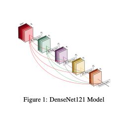
In order to maximize the information flow through shortcuts between layers while using less VM capacity than a traditional deep CNN, we used a DenseNet121 architecture. The DenseNet121 served as our baseline for accuracy because the Stanford group found it to be most accurate model for the CheXpert dataset. In this model, the input tensor first flows through a convolutional feature layer to capture low-level features of the X-ray such as lines, colors, and boundaries. This is followed by a series of four dense blocks with transition layers in between. These dense blocks have 6, 12, 24, and 16 layers layers of alternating Batchnorm, ReLu, and 2D Convolutions. The output of the DenseNet121 was passed into a logistic classifier to generate final diagnostic predictions.

6.2 VGG19 and VGG16
We utilized VGG19 and VGG16 because we were interested if we could build
upon Nair et al.’s group’s promising but inconclusive results when using these architectures. The VGG network is a neural network that has already been pretrained on over a million images from the ImageNet database. The network applies multi-scale training, which may be helpful for our task because our x-rays are non-uniform. If the network is only trained on one scale, it might misclassify x-rays of other scales. Furthermore, the VGG networks have also performed very well on a variety of image classification tasks. Our VGG16 is composed of 16 convolutional layers and VGG19 adds on another 3 fully connected layers to the end. These networks have a considerable number of parameters, so its training process is quite slow.
6.3 Kernelized SVMs using DenseNet as Feature Extractor
The success of Saad, Mohd Nizam et al.’s research in using an SVM kernel for nodule location chest X-ray classification inspired us to implement the linear, polynomial and RBF SVMs to determine if their success in the nodule location task generalizes to our disease diagnosis task. For feature extraction, we passed our x-rays into a vanilla pre-trained DenseNet121 to obtain a feature vector of size 1,024, which is typically the number of features used in the DenseNet architecture to perform classification. We specifically decided to implement a linear SVM because its hinge loss is less sensitive to outliers and will work better than the baseline DenseNet that uses a logistic classifier in the case that our has some outliers. We suspect that this might be the case since our dataset consists of non-uniform x-ray images. In addition, we decided to implement the polynomial SVM and an radial basis SVM because they are high performing non-linear classifiers, and in the case that our data is best separated by a non-linear boundary, using one of these kernelized SVMs will improve performance.
6.4 Decision Tree using DenseNet as Feature Extractor
We decided to implement a decision tree with features from DenseNet for two main reasons. The first reason is that the Decision Tree is a high performing non-linear classifier that may improve performance on our task, if a non-linear boundary best separates our data. The second reason was inspired by Nair, Aditya et al.’s Interpreting CNNs via Decision Trees. Nair, Aditya et al demonstrated that the decision tree algorithm can be used to interpret the how much each CNN feature contributes to making a final prediction. Since, our main task is clinically focused, one of our secondary goals was to implement this decision tree classifier and open source it, in the case that it might be useful to certain medical professionals to know which features contribute the most a certain diagnosis.
7 Results
7.1 VGG16 and VGG19
The VGG16 and VGG19 architectures did not perform as well as our DenseNet baseline, despite having high performance on a variety of other image classification tasks. Using the mean AUROC score as our evaluation metric, DenseNet121 outperformed both VGG19 and VGG16 on all three view types. These gains are likely due to the DenseNet’s ability to directly leverage earlier layers. This strengthens feature propagation and encourage feature reuse which is crucial because disease diagnoses can stem from tiny changes within the images. It also avoids the vanishing gradient problem that VGG networks run into.

7.2 Polynomial SVM and Radial Basis Function SVM using DenseNet as Feature Extractor
Our linear SVM classifier using DenseNet extracted features slightly outperformed the vanilla DenseNet baseline that uses a logistic
classifer as its final layer. This improvement in performance is most likely due to the difference in the loss functions of the two classifiers. As previously mentioned, X-ray scans are not uniform in scale and may have some outliers. The Linear SVM utilizes a hinge loss function that is less sensitive to outliers in the data, which may explain why it outperforms the logistic classifier for this particular task. We used a cost factor of 1 and a gamma value of 1.
7.3 Polynomial SVM and Radial Basis Function SVM using DenseNet as Feature Extractor
Our polynomial and RBF SVMs using DenseNet extracted features made further improvements upon the linear SVM classifier and the vanilla DenseNet baseline. Because all of these classifiers use the same features from DenseNet, the fact that the polynomial and RBF SVMs have better performance suggests that non-linear decision boundaries may be better at separating out this particular dataset. We used a cost factor of 1 and a gamma value of 1.
7.4 Decision Tree using DenseNet as Feature Extractor
The decision tree using DenseNet as a feature extractor was our best performing model overall. Similar to what was previously mentioned,
since all the model classifiers use the same features from DenseNet, the reason why the decision tree performed the best is most likely because of the way it draws decision boundaries. The decision tree cuts up the space based on information gain, in which the most expressive features are first used to separate out the data followed by the less expressive features. We used a max depth of 32, minimum sample leaves of 5 and 100 random states.
7.5 View-Specific Models: Results and Analysis
When tested on a dataset with all view types, the DenseNet121 and VGG19 baselines trained on all views outperformed our view-specific
models.

Our view-specific models that obtain view labels with our CNN view classifier had comparable results to the view-specific models given the ground-truth labels. This result falls in line with our expectations for two reasons. First, we had very high accuracy with our CNN view-classifier so we would not expect many scans to have a mis-classified view type. Second, the strong results of our baseline lead us to believe that view-specific models can fairly accurately classify X-ray scans of a different view type. Therefore, mis-classifying a scan and thus using the wrong view-specific model for classification only leads to a marginal decrease in classification accuracy.
We hypothesize that the strong performance of the baseline is because the different view types are similar enough that one model is sufficient to effectively learn and classify different view types. Features learned from frontal scans can help in classification on lateral scans. Additionally, it seems that we lacked training data for the lateral and PA views. This hypothesis is supported by how 72 percent of all view data is of view-type AP.
To test this hypothesis, we evaluated the view-specific models on a dataset comprised of X-ray scans taken only from the view type that the view-specific model was trained on (Table 3). We see every individual view-specific model is out-performed by the baseline. This also leads us to believe that the poor performance of the view-specific models is due to the fact that all view-specific models had less training data than the baseline.

As expected, the view-specific model for AP was closest to performing at the baseline level. The near-baseline performance of the our AP view-specific model leads us to reach a fairly intuitive conclusion: If we had trained the AP view-specific model on a AP-only dataset of equal size to the baseline’s mixed-view data, the AP view-specific model would outperform the baseline. However, our research indicates view-specific modeling and training is unlikely to lead to significant advances in classification accuracy.
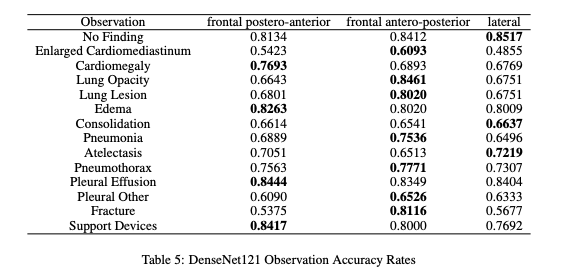
We further broke down our results by examining the results of our baseline DenseNet model (trained on all view types) on three test sets, one for each view type. Then, we examined the results of this test on the level of prediction accuracies for each chest observation (presence of chest conditions/diseases). The model tested on frontal AP performs best for 7/14 observations while the model tested on PA performs best for 4/14 observations and the model tested on lateral performs best for 3/14 observations. Among the observations that were best classified on the AP dataset, the tests have an average improvement of 10.27 percent compared to the next best view. Meanwhile the average improvement for frontal PA and lateral views were 3.75 and 1 percent respectively. This discrepancy in performance corresponds closely to the distribution of our data. AP views account for 72 percent of the data, PA views account for 13 percent of the data and lateral views account for 15 percent of the data.

However, training on specific views performed similarly well on AP and worse the PA and lateral test sets than on our models trained on all views. This decrease in performance is likely because when testing lateral X-rays, training the model on frontal X-rays does not cause the model to learn conflicting information. PA and lateral x-rays represent a minority of our dataset and limiting the training set to one view type decreased our amount of training data and hurt our model.
8 Conclusion
We have managed to greatly improve upon our baseline AUROC score from .76 to .93. We did this by replacing DenseNet’s final layer of a logistic classifier with a Decision Tree. This is likely because nonlinear decision boundaries better fit our data than linear decision boundaries. Meanwhile, our attempts to train specialized disease classification models failed to improve upon our baseline on all view types. After examining results at a view-type and observation level, we hypothesize that these poor results are primarily due to a lack of training data. Additionally, we see that scans of different view types are similar enough that view-specific models can benefit from learning from any scan.
We recognize that our training data was heavily composed of AP views. In the future, we wish to expand the number of chest X-rays
taken from the PA and lateral views in our training set. This would allow us gather more precise weightings for the importance of views.
In addition, if we had more time, we would also like to perform uncertainty analysis to quantify the variability of our output in cases
where chest X-rays taken from different views in the same study had conflicting predictions. This would give allow us to inform users on
the uncertainty of our prediction.
9 Individual Contributions
9.1 Danny Takeuchi
Researched existing papers and code repositories that utilized the CheXpert dataset. Programmed logistic regression and a feed forward
neural network view classifiers and the initial DenseNet/VGG baselines. Created the test sets for each view, generated the visual aids, and
conducted error analysis. Drafted up most of the paper and poster.
9.2 Raymond Thai
Implemented patient/study grouping, researched model architectures, researched image classification papers, cleaned data, generated
datasets, designed and conducted most tests for view-specific models, and conducted error analysis.
9.3 Kevin Tran
Wrote CNN view classifier, incorporated CNN view classifier with existing training pipeline, implemented the various SVMs and the
decision tree, analyzed results for different model architectures and set up cloud environments.
10 References
Our Github Repository: https://github.com/danny-takeuchi/cs229_CheXpert
1. Bar, Yaniv, et al. “Chest pathology detection using deep learning with non-medical training.” 2015 IEEE 12th International
Symposium on Biomedical Imaging (ISBI). IEEE, 2015.
2. Huang, Gao, et al. “Densely connected convolutional networks.” Proceedings of the IEEE conference on computer vision and
pattern recognition. 2017.
3. Irvin, Jeremy, et al. “Chexpert: A large chest radiograph dataset with uncertainty labels and expert comparison.” Thirty-Third
AAAI Conference on Artificial Intelligence. 2019.
4. Saad MN, Muda Z, Sahari @ Ashaari N, Abdul Hamid H. Multiclass classification application using SVM kernel to classify chest
X-ray images based on nodule location in lung zones. Journal of Telecommunication, Electronic and Computer Engineering.
2017;9(1–2):19–23.
5. Nair, Aditya, et al. “Detection of Diseases on Chest X-ray Using Deep Learning.” 2019.
6. Zhang, Quanshi, et al. “Interpreting CNNs via decision trees.” arXiv preprint arXiv:1802.00121. 2018.
7. https://github.com/kshitij0987
8. https://stanfordmlgroup.github.io/competitions/chexpert/


