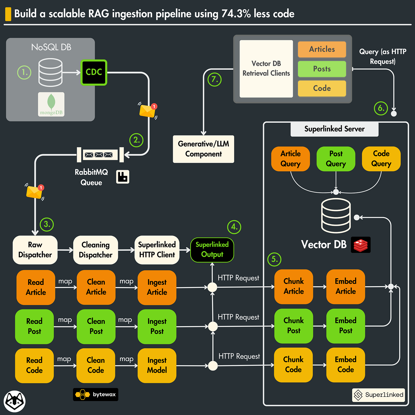
Build a scalable RAG ingestion pipeline using 74.3% less code
Welcome to Lesson 11 of 12 in our free course series, LLM Twin: Building Your Production-Ready AI Replica. You’ll learn how to use LLMs, vector DVs, and LLMOps best practices to design, train, and deploy a production ready “LLM twin” of yourself. This AI character will write like you, incorporating your style, personality, and voice into an LLM. For a full overview of course objectives and prerequisites, start with Lesson 1.
Lessons
- An End-to-End Framework for Production-Ready LLM Systems by Building Your LLM Twin
- Your Content is Gold: I Turned 3 Years of Blog Posts into an LLM Training
- I Replaced 1000 Lines of Polling Code with 50 Lines of CDC Magic
- SOTA Python Streaming Pipelines for Fine-tuning LLMs and RAG — in Real-Time!
- The 4 Advanced RAG Algorithms You Must Know to Implement
- Turning Raw Data Into Fine-Tuning Datasets
- 8B Parameters, 1 GPU, No Problems: The Ultimate LLM Fine-tuning Pipeline
- The Engineer’s Framework for LLM & RAG Evaluation
- Beyond Proof of Concept: Building RAG Systems That Scale
- The Ultimate Prompt Monitoring Pipeline
- [Bonus] Build a scalable RAG ingestion pipeline using 74.3% less code
- [Bonus] Build Multi-Index Advanced RAG Apps
Lessons 11 and 12 are part of a bonus series in which we will take the advanced RAG system from the LLM Twin course (written in LangChain) and refactor it using Superlinked, a framework specialized in vector computing for information retrieval.
In Lesson 11 (this article), we will learn to build a highly scalable, real-time RAG feature pipeline that ingests multi-data categories into a Redis vector database.
More concretely we will take the ingestion pipeline implemented in Lesson 4 and swap the chunking, embedding, and vector DB logic with Superlinked.
You don’t have to read Lesson 4 to read this article. We will give enough context to make sense of it.
In the 12th lesson, we will use Superlinked to implement a multi-index query strategy and further optimize the advanced RAG retrieval module (initially built in Lesson 5).
The value of this article lies in understanding how easy it is to build complex advanced RAG systems using Superlinked.
Using Superlinked, we reduced the number of RAG-related lines of code by 74.3%. Powerful, right?
By the end of this article, you will learn to build a production-ready feature pipeline built in Superlinked that:
- uses Bytewax as a stream engine to process data in real-time;
- ingests multiple data categories from a RabbitMQ queue;
- validates the data with Pydantic;
- chunks, and embeds data using Superlinked for doing RAG;
- loads the embedded vectors along their metadata to a Redis vector DB;
Ultimately, on the infrastructure side, we will show you how to:
- deploy a Superlinked vector compute server;
- Dockerize the RAG ecosystem.
Note: In our use case, the feature pipeline is also a streaming pipeline, as we use a Bytewax streaming engine. Thus, we will use these words interchangeably.
Quick intro in feature pipelines
The feature pipeline is the first pipeline presented in the FTI pipeline architecture: feature, training and inference pipelines.
A feature pipeline takes raw data as input, processes it into features, and stores it in a feature store, from which the training & inference pipelines will use it.
The component is completely isolated from the training and inference code. All the communication is done through the feature store.
To avoid repeating myself, if you are unfamiliar with the FTI pipeline architecture, check out Lesson 1 for a refresher.
Table of Contents
- What is Superlinked?
- The old architecture of the RAG feature pipeline
- The new Superlinked architecture of the RAG feature pipeline
- Understanding the streaming flow for real-time processing
- Loading data to Superlinked
- Exploring the RAG Superlinked server
- Using Redis as a vector DB
- Dockerize the application
🔗 Check out the code on GitHub [1] and support us with a ⭐️
1. What is Superlinked?
Superlinked is a computing framework for turning complex data into vectors.
It lets you quickly build multimodal vectors and define weights at query time, so you don’t need a custom reranking algorithm to optimize results.
Superlinked focuses on solving complex problems based on vector embeddings, such as RAG, semantic search, and recommendation systems.
I love how Daniel Svonava, the CEO of Superlinked, described the value of vector compute and implicitly Superlinked:
Daniel Svonava, CEO at Superlinked:
“Vectors power most of what you already do online — hailing a cab, finding a funny video, getting a date, scrolling through a feed or paying with a tap. And yet, building production systems powered by vectors is still too hard! Our goal is to help enterprises put vectors at the center of their data & compute infrastructure, to build smarter and more reliable software.”
To conclude, Superlinked is a framework that puts the vectors in the center of their universe and allows you to:
- chunk and embed embeddings;
- store multi-index vectors in a vector DB;
- do complex vector search queries on top of your data.
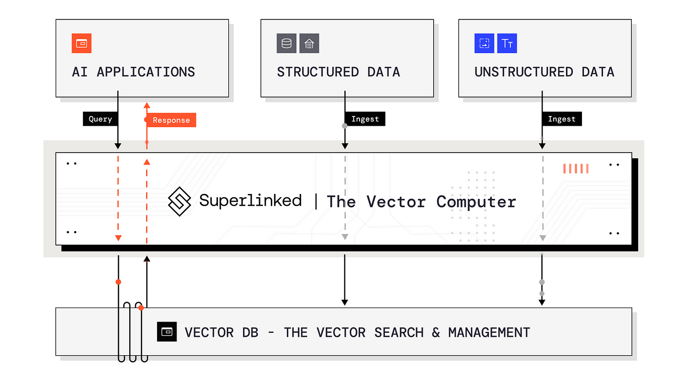
Screenshot from Superlinked’s landing page
Superlinked vs LangChain (or LlamaIndex)
Superlinked solely specializes in vector computing (chunking, embedding, vector DBs and vector searches). It is a highly specialized knife for “cutting” vectors.
On the other hand, frameworks such as LangChain or LlamaIndex are like Swiss Army Knives, able to do almost everything related to LLM applications.
Because of their fast number of features, they couldn’t specialize in a specific niche, such as vector computing.
Any framework would do the trick for a quick PoC, but Superlinked will make a difference when working with complex data structures that require multi-indexing and complicated queries.
Also, as a personal note, I love how simple and intuitive Superlinked’s Python SDK is compared to other frameworks.
2. The old architecture of the RAG feature pipeline
Here is a quick recap of the critical aspects of the architecture of the RAG feature pipeline presented in the 4th lesson of the LLM Twin course.
We are working with 3 different data categories:
- posts (e.g., LinkedIn, Twitter)
- articles (e.g., Medium, Substack, or any other blog)
- repositories (e.g., GitHub, GitLab)
Every data category has to be preprocessed differently. For example, you want to chunk the posts into smaller documents while keeping the articles in bigger ones.
The solution is based on CDC, a queue, a streaming engine, and a vector DB:
-> The raw data is collected from multiple social platforms and is stored in MongoDB. (Lesson 2)
→ CDC adds any change made to the MongoDB to a RabbitMQ queue (Lesson 3).
→ the RabbitMQ queue stores all the events until they are processed.
→ The Bytewax streaming engine reads the messages from the RabbitMQ queue and cleans, chunks, and embeds them.
→ The processed data is uploaded to a Qdrant vector DB.
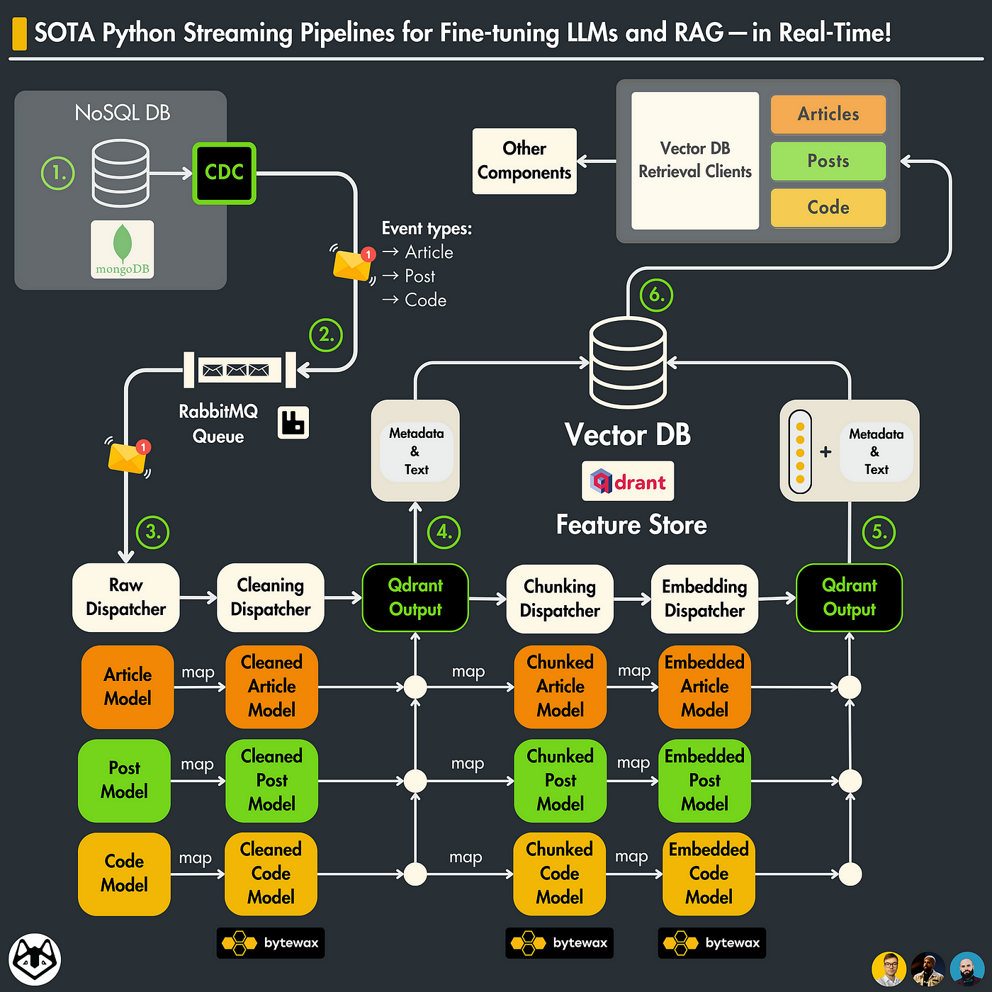
Why is this design robust?
Here are 4 core reasons:
- The data is processed in real-time.
- Out-of-the-box recovery system: If the streaming pipeline fails to process a message, it will be added back to the queue
- Lightweight: No need for any diffs between databases or batching too many records
- No I/O bottlenecks on the source database
We recommend reading (or at least skimming) Lesson 4 to understand the details of the old streaming architecture.
What is the issue with this design?
In this architecture, we had to write custom logic to chunk, embed, and load the data to Qdrant.
The issue with this approach is that we had to leverage various libraries, such as LangChain and unstructured, to get the job done.
Also, because we have 3 data categories, we had to write a dispatcher layer that calls the right function depending on its category, which resulted in tons of boilerplate code.
Ultimately, as the chunking and embedding logic is implemented directly in the streaming pipeline, it is harder to scale horizontally. The embedding algorithm needs powerful GPU machines, while the rest of the operations require a strong CPU.
This results in:
- more time spent on development;
- more code to maintain;
- the code can quickly become less readable;
- less freedom to scale.
Superlinked can speed up this process by providing a very intuitive and powerful Python API that can speed up the development of our ingestion and retrieval logic.
Thus, let’s see how to redesign the architecture using Superlinked ↓
3. The new Superlinked architecture of the RAG feature pipeline
The core idea of the architecture will be the same. We still want to:
- use a Bytewax streaming engine for real-time processing;
- read new events from RabbitMQ;
- clean, chunk, and embed the new incoming raw data;
- load the processed data to a vector DB.
The question is, how will we do this with Superlinked?
As you can see in the image below, Superlinked will replace the logic for the following operations:
- chunking;
- embedding;
- vector storage;
- queries.
Also, we have to swap Qdrant with a Redis vector DB because Superlinked didn’t support Qdrant when I wrote this article. But they plan to add it in future months (along with many other vector DBs).
What will remain unchanged are the following:
- the Bytewax streaming layer;
- the RabbitMQ queue ingestion component;
- the cleaning logic.
By seeing what we must change to the architecture to integrate Superlinked, we can see the framework’s core features.
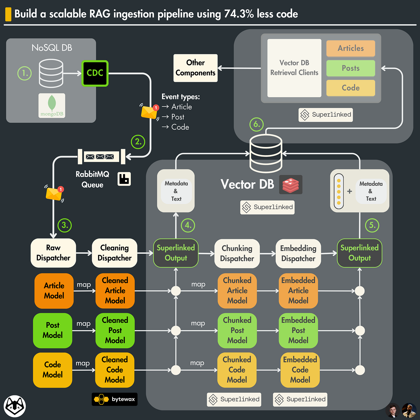
Now, let’s take a deeper look at the new architecture.
All the Superlinked logic will sit on its own server, completely decoupling the vector compute component from the rest of the feature pipeline.
We can quickly scale the streaming pipeline or the Superlinked server horizontally based on our needs. Also, this makes it easier to run the embedding models (from Superlinked) on a machine with a powerful GPU while keeping the streaming pipeline on a machine optimized for network I/O operations.
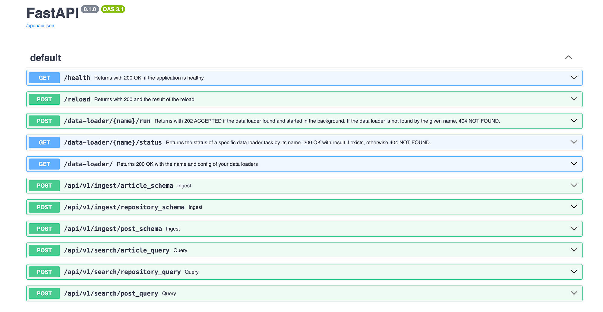
All the communication to Superlinked (ingesting or query data) will be done through a REST API, automatically generated based on the schemas and queries you define in your Superlinked application.
The Bytewax streaming pipeline will perform the following operations:
- will concurrently read messages from RabbitMQ;
- clean each message based on it’s data category;
- send the cleaned document to the Superlinked server through an HTTP request.
On the Superlinked server side, we have defined an ingestion endpoint for each data category (article, post or code). Each endpoint will know how to chunk embed and store every data point based on its category.
Also, we have a query endpoint (automatically generated) for each data category that will take care of embedding the query and perform a vector semantic search operation to retrieve similar results.

Now, let’s finally jump into the code ↓
4. Understanding the streaming flow for real-time processing
Let’s start with a quick recap of the Bytewax streaming flow we presented in Lesson 4 in more detail.
The Bytewax flow is the central point of the streaming pipeline. It defines all the required steps, following the next simplified pattern: “input -> processing -> output”.
To structure and validate the data, we use Pydantic. Between each Bytewax step, we map and pass a different Pydantic model based on its current state: raw, cleaned, chunked, or embedded.
If we get an invalid data point due to contract changes between the feature pipeline and the events coming from RabbitMQ, instead of having side effects in the system, Pydantic will throw an error. Thus, we can quickly react instead of having silent failures or other side effects.
Here is the Bytewax flow and its core steps ↓
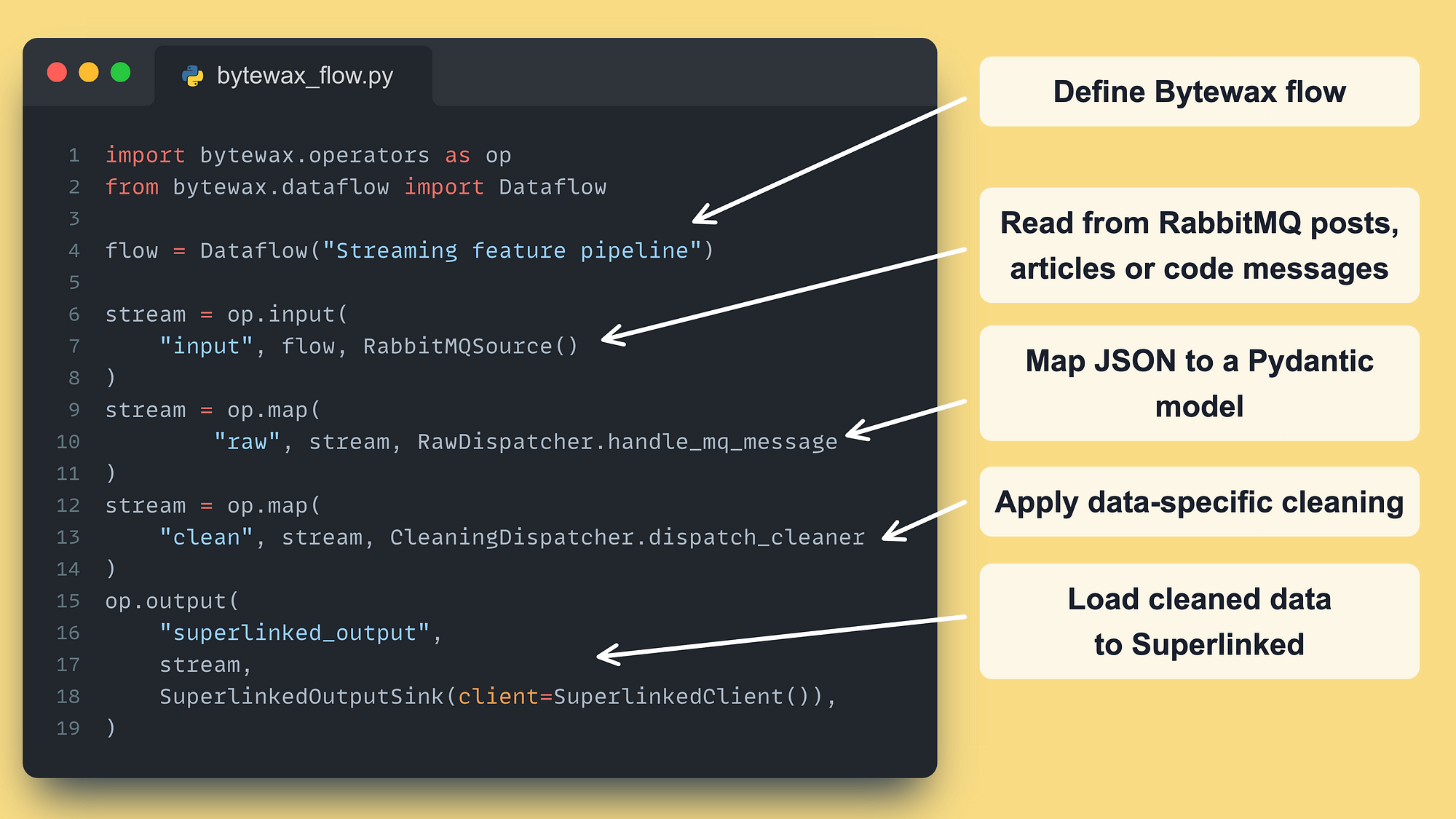
Check out Lesson 4 for more details on the Bytewax flow, how the map() functions work and how the data is clean. This lesson will primarily focus on Superlinked and how to write an RAG feature pipeline with it.
What is important to remain with is that once a message is available in the RabbitMQ queue, it will immediately be:
- consumed;
- transformed to a raw Pydantic model (Pydantic automatically validates the structure and data types);
- cleaned;
- sent to the Superlinked server to be chunked, embedded and saved to a vector DB.
5. Loading data to Superlinked
Before we explore the Superlinked application, let’s review our Bytewax SuperlinkedOutputSink() and SuperlinkedClient() classes.
The SuperlinkedOutputSink() class inherits the DynamicSink base class from Bytewax, which implements output nodes in a flow.
Its purpose is to instantiate a new SuperlinkedSinkPartition() for each worker within the Bytewax cluster. Thus, we can optimize the system for I/O operations by scaling our output workers horizontally.
 class SuperlinkedOutputSink(DynamicSink):
    def __init__(self, client: SuperlinkedClient) -> None:
        self._client = client

    def build(self, worker_index: int, worker_count: int) -> StatelessSinkPartition:
        return SuperlinkedSinkPartition(client=self._client)
The SuperlinkedSinkPartition() class inherits the StatelessSinkPartition Bytewax base class used to create custom stateless partitions. Each partition will run on a different worker. As they are stateless, you can directly spin up new workers when required.
This class takes as input batches of items and sends them to Superlinked through the SuperlinkedClient().
 class SuperlinkedSinkPartition(StatelessSinkPartition):
    def __init__(self, client: SuperlinkedClient):
        self._client = client

    def write_batch(self, items: list[Document]) -> None:
        for item in tqdm(items, desc="Sending items to Superlinked..."):
            match item.type:
                case "repositories":
                    self._client.ingest_repository(item)
                case "posts":
                    self._client.ingest_post(item)
                case "articles":
                    self._client.ingest_article(item)
                case _:
                    logger.error(f"Unknown item type: {item.type}")
The SuperlinkedClient() is a basic wrapper that makes HTTP requests to the Superlinked server that contains all the RAG logic. We use httpx to make POST requests for ingesting or searching data.
We will use this class to communicate between:
- the RAG feature pipeline -> Superlinked server (when ingesting data)
- the RAG retriever <-> Superlinked server (when retrieving data for passing it to an LLM)
 class SuperlinkedClient:
    def __init__(self, base_url=settings.SUPERLINKED_SERVER_URL) -> None:
        self.base_url = base_url
        self.timeout = 600
        self.headers = {"Accept": "*/*", "Content-Type": "application/json"}

        self._content_weight = 0.9
        self._platform_weight = 0.1

    def ingest_repository(self, data: RepositoryDocument) -> None:
        self.__ingest(f"{self.base_url}/api/v1/ingest/repository_schema", data)

    def ingest_post(self, data: PostDocument) -> None:
        self.__ingest(f"{self.base_url}/api/v1/ingest/post_schema", data)

    def ingest_article(self, data: ArticleDocument) -> None:
        self.__ingest(f"{self.base_url}/api/v1/ingest/article_schema", data)

    def __ingest(self, url: str, data: T) -> None:
        logger.info(f"Sending article {data.id} to Superlinked at {url}")

        response = httpx.post(
            url, headers=self.headers, json=data.model_dump(), timeout=self.timeout
        )

        if response.status_code != 202:
            raise httpx.HTTPStatusError(
                "Ingestion failed", request=response.request, response=response
            )

    def search_repository(
        self, search_query: str, platform: str, author_id: str, *, limit: int = 3
    ) -> list[RepositoryDocument]:
        return self.__search(
            f"{self.base_url}/api/v1/search/repository_query",
            RepositoryDocument,
            search_query,
            platform,
            author_id,
            limit=limit,
        )

    def search_post(
        self, search_query: str, platform: str, author_id: str, *, limit: int = 3
    ) -> list[PostDocument]:
        ... # URL: f"{self.base_url}/api/v1/search/post_query"

    def search_article(
        self, search_query: str, platform: str, author_id: str, *, limit: int = 3
    ) -> list[ArticleDocument]:
        ... # URL: f"{self.base_url}/api/v1/search/article_query"

    def __search(
        self,
        url: str,
        document_class: type[T],
        search_query: str,
        platform: str,
        author_id: str,
        *,
        limit: int = 3,
    ) -> list[T]:
        url = f"{self.base_url}/api/v1/search/repository_query"

        data = {
            "search_query": search_query,
            "platform": platform,
            "author_id": author_id,
            "limit": limit,
            "content_weight": self._content_weight,
            "platform_weight": self._platform_weight,
        }
        response = httpx.post(
            url, headers=self.headers, json=data, timeout=self.timeout
        )

        if response.status_code != 200:
            raise httpx.HTTPStatusError(
                "Search failed", request=response.request, response=response
            )

        parsed_results = []
        for result in response.json()["results"]:
            parsed_results.append(document_class(**result["obj"]))

        return parsed_results
The Superlinked server URLs are automatically generated as follows:
- The ingestion URLs are generated based on the data schemas you defined (e.g., repository schema, post schema, etc.)
- The search URLs are created based on the Superlinked queries defined within the application
If that doesn’t make sense, it will in just a second after we go through the Superlinked application ↓
6. Exploring the RAG Superlinked server
As the RAG Superlinked server is a different component than the Bytewax one, the implementation sits under the server folder at 6-bonus-superlinked-rag/server/src/app.py.
Under the hood, Superlinked uses FastAPI to bootstrap a web server over its core engine. You won’t have to interact with FastAPI, but it’s good to know as you leverage its features, such as the Swagger UI [2] for documentation, which you can access at /docs:
Settings class
Use Pydantic settings to define a global configuration class.
 class Settings(BaseSettings):
    EMBEDDING_MODEL_ID: str = "sentence-transformers/all-mpnet-base-v2"

    REDIS_HOSTNAME: str = "redis"
    REDIS_PORT: int = 6379


settings = Settings()
Schemas
Superlinked requires you to define your data structure through a set of schemas, which are very similar to data classes or Pydantic models.
Superlinked will use these schemas as ORMs to save your data to a specified vector DB.
It will also use them to define ingestion URLs automatically as POST HTTP methods that expect the request body to have the same signature as the schema.
Simple and effective. Cool, right?
 @schema
class PostSchema:
    id: IdField
    platform: String
    content: String
    author_id: String
    type: String


@schema
class ArticleSchema:
    id: IdField
    platform: String
    link: String
    content: String
    author_id: String
    type: String


@schema
class RepositorySchema:
    id: IdField
    platform: String
    name: String
    link: String
    content: String
    author_id: String
    type: String


post = PostSchema()
article = ArticleSchema()
repository = RepositorySchema()
There is nothing fancy here. Let’s move to Superlinked’s coolest feature, spaces.
Spaces
The spaces are where you define your chunking and embedding logic.
A space is scoped at the field of a schema. Thus, if you want to embed multiple attributes of a single schema, you must define multiple spaces and combine them later into a multi-index.
Let’s take the spaces for the article category as an example:
 articles_space_content = TextSimilaritySpace(
    text=chunk(article.content, chunk_size=500, chunk_overlap=50),
    model=settings.EMBEDDING_MODEL_ID,
)
articles_space_plaform = CategoricalSimilaritySpace(
    category_input=article.platform,
    categories=["medium", "superlinked"],
    negative_filter=-5.0,
)
Chunking is done simply by calling the chunk() function on a given schema field and specifying standard parameters such as “chunk_size” and “chunk_overlap”.
The embedding is done through the TextSimilaritySpace() and CategoricalSimilaritySpace() classes.
As the name suggests, the TextSimilaritySpace() embeds text data using the model specified within the “model” parameter. It supports any HuggingFace model. We are using “sentence-transformers/all-mpnet-base-v2”.
The CategoricalSimilaritySpace() class uses an n-hot encoded vector with the option to apply a negative filter for unmatched categories, enhancing the distinction between matching and non-matching category items.
The “negative_filter” parameter allows for the filtering out of unmatched categories by setting them to a large negative value, effectively resulting in a large negative similarity between non-matching category items.
You must also specify all the available categories through the “categories” parameter to encode them in n-hot.
As you can see in the GitHub repository, the spaces for the repository and posts look exactly the same.
Indexes
The indexes define how a collection can be queried. They take one or multiple spaces from the same schema.
Here is what the article index looks like:
 article_index = Index(
    [articles_space_content, articles_space_plaform],
    fields=[article.author_id],
)
As you can see, the vector index combines the article’s content and the posted platform. When the article collection is queried, both embeddings will be considered.
Also, we index the “author_id” field to filter articles written by a specific author. It is nothing fancy—it is just a classic filter. However, indexing the fields used in filters is often good practice.
The repository and post indexes look the same, as you can see in the GitHub repository.
Queries
We will quickly introduce what a query looks like. But in the 12th lesson, we will insist on the advanced retrieval part, hence on queries.
Here is what the article query looks like:
 article_query = (
    Query(
        article_index,
        weights={
            articles_space_content: Param("content_weight"),
            articles_space_plaform: Param("platform_weight"),
        },
    )
    .find(article)
    .similar(articles_space_content.text, Param("search_query"))
    .similar(articles_space_plaform.category, Param("platform"))
    .filter(article.author_id == Param("author_id"))
    .limit(Param("limit"))
)
…and here is what it does:
- it queries the article_index using a weighted multi-index between the content and platform vectors (e.g.,
0.9 * content_embedding + 0.1 * platform_embedding); - the search text used to compute query content embedding is specified through the “search_query” parameter and similar for the platform embedding through the “platform” parameter;
- we filter the results based on the “author_id”;
- take only the top results using the “limit” parameter.
These parameters are automatically exposed on the REST API endpoint, as seen in the SuperlinkedClient() class.
Sources
The sources wrap the schemas and allow you to save that schema in the database.
In reality, the source maps the schema to an ORM and automatically generates REST API endpoints to ingest data points.
article_source = RestSource(article) Executor
The last step is to define the executor that wraps all the sources, indices, queries and vector DB into a single entity:
 executor = RestExecutor(
    sources=[article_source, repository_source, post_source],
    indices=[article_index, repository_index, post_index],
    queries=[
        RestQuery(RestDescriptor("article_query"), article_query),
        RestQuery(RestDescriptor("repository_query"), repository_query),
        RestQuery(RestDescriptor("post_query"), post_query),
    ],
    vector_database=InMemoryVectorDatabase(),
)
Now, the last step is to register the executor to the Superlinked engine:
SuperlinkedRegistry.register(executor) …and that’s it!
Joking… there is something more. We have to use a Redis database instead of the in-memory one.
7. Using Redis as a vector DB
First, we have to spin up a Redis vector database that we can work with.
We used Docker and attached a Redis image as a service in a docker-compose file along with the Superlinked poller and executor (which comprise the Superlinked server):
 version: "3"

services:
  poller:
    ...

  executor:
    ...

  redis:
    image: redis/redis-stack:latest
    ports:
      - "6379:6379"
      - "8001:8001"
    volumes:
      - redis-data:/data

volumes:
  redis-data:
Now, Superlinked makes everything easy. The last step is to define a RedisVectorDatabase connector provided by Superlinked:
 vector_database = RedisVectorDatabase(
    settings.REDIS_HOSTNAME,  # (Mandatory) This is your redis URL without any port or extra fields
    settings.REDIS_PORT,  # (Mandatory) This is the port and it should be an integer
)
…and swap it in the executor with the InMemoryVectorDatabase() one:
 executor = RestExecutor(
    ...
    vector_database=vector_database,
)
As we are using the “redis-stack” Docker image, you can visualize everything inside Redis at http://localhost:8001/redis-stack/browser.

Now we are done!
We have created a Superlinked server that:
- chunks and embeds every data category differently;
- writes all the ingested data to a Redis vector DB;
- can ingest and query articles, posts and repositories;
- support multi-index vector search between the content and the platform of the data point;
- has ingestion and search REST API endpoints;
…and all of that in only 486 lines of code. Pretty cool, right?
8. Dockerize the application
The article is already too long.
Thus, we won’t get into the details of Dockerization, but we want to let you know that the repository supports Docker.
Here is where you can find all the Docker and Docker compose files required to run the RAG feature pipeline and Superlinked server:
- Bytewax Docker image;
- LLM Twin system docker-compose file;
- Superlinked server docker-compose file (where the Redis database is defined).
→ The GitHub repository provides step-by-step details on building and starting the Docker images to run the whole project. ←
Conclusion
Congratulations! You learned to write advanced RAG systems using Superlinked.
More concretely, in Lesson 11, you learned:
- what is Superlinked;
- how to design a streaming pipeline using Bytewax;
- how to design a RAG server using Superlinked;
- how to take a standard RAG feature pipeline and refactor it using Superlinked;
- how to split the feature pipeline into 2 services, one that reads in real-time messages from RabbitMQ and one that chunks, embeds, and stores the data to a vector DB;
- how to use a Redis vector DB.
Lesson 12 will teach you how to implement multi-index queries to optimize the RAG retrieval layer further.
🔗 Check out the code on GitHub [1] and support us with a ⭐️
→ Also, if curious, check out Superlinked to learn more about them.
References
Literature
[1] Your LLM Twin Course — GitHub Repository (2024), Decoding ML GitHub Organization
[2] Swagger UI, FastAPI documentation
[3] Superlinked Demo Notebook, Google Colab
[4] Superlinked Server, Superlinked GitHub repository
[5] Superlinked Redis Example, Superlinked GitHub repository
[6] Superlinked RAG Example, Superlinked GitHub repository
Images
If not otherwise stated, all images are created by the author.

