Random Forest Regression in Python Using Scikit-Learn

Introduction
A random forest is an ensemble model that consists of many decision trees. Predictions are made by averaging the predictions of each decision tree. Or, to extend the analogy—much like a forest is a collection of trees, the random forest model is also a collection of decision tree models. This makes random forests a strong modeling technique that’s much more powerful than a single decision tree.
Each tree in a random forest is trained on the subset of data provided. The subset is obtained both with respect to rows and columns. This means each random forest tree is trained on a random data point sample, while at each decision node, a random set of features is considered for splitting.
In the realm of machine learning, the random forest regression algorithm can be more suitable for regression problems than other common and popular algorithms. Below are a few cases where you’d likely prefer a random forest algorithm over other regression algorithms:
- There are non-linear or complex relationships between features and labels.
- You need a model that’s robust, meaning its dependence on the noise in the training set is limited. The random forest algorithm is more robust than a single decision tree, as it uses a set of uncorrelated decision trees.
- If your other linear model implementations are suffering from overfitting, you may want to use a random forest.
A bit more about point 3. Decision trees are prone to overfitting, especially if we don’t limit the max depth—they have unlimited flexibility, and hence can keep growing until they have exactly one leaf node for every single data point, thus perfectly predicting all of them.
When we limit the max depth of a decision tree, the variance is reduced, but bias increases. To keep both variance and bias low, the random forest algorithm combines many decision trees with randomness to reduce overfitting.
Before we jump into an implementation of random forest for a regression problem, let’s define some key terms.
Key Terms
Bootstrapping
This is the process of sampling data, where you draw a sample data point out of a population, measure the sample, and return the sample back to the population, before drawing the next sample point.
For example, out of the n data points given, s sample data points are chosen with replacement. We train decision trees on each of these sample. Sampling with replacement is used to make the resampling a random event. If we do resampling without replacement, the samples drawn will be dependent on the previous ones and thus not be random.
It is worth noting that as samples are drawn with replacement, some samples may be used multiple times in a single tree.
Bagging
Random forests train each individual decision tree on different bootstrapped samples of the data, and then average the predictions to make an overall prediction. This is called bagging.
Implementation
Now let’s start our implementation using Python and a Jupyter Notebook.
Once the Jupyter Notebook is up and running, the first thing we should do is import the necessary libraries.
We need to import:
- NumPy
- Pandas
- RandomForestRegressor
- train_test_split
- r2_score
- mean squared error
- Seaborn
To actually implement the random forest regressor, we’re going to use scikit-learn, and we’ll import our RandomForestRegressor from sklearn.ensemble.
import numpy as np
import pandas as pd
from sklearn.model_selection import train_test_split
from sklearn.ensemble import RandomForestRegressor
from sklearn.metrics import r2_score,mean_squared_error
import seaborn as sns
Load the Data
Once the libraries are imported, our next step is to load the data, stored here. You can download the data and keep it in your local folder. After that we can use the read_csv method of Pandas to load the data into a Pandas data frame df, as shown below.
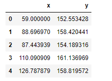
Also shown in the snapshot of the data below, the data frame has two columns, x and y. Here, x is the feature and y is the label. We’re going to predict y using x as an independent variable.
df = pd.read_csv(‘Random-Forest-Regression-Data.csv’)

Data pre-processing
Before feeding the data to the random forest regression model, we need to do some pre-processing.
Here, we’ll create the x and y variables by taking them from the dataset and using the train_test_split function of scikit-learn to split the data into training and test sets.
We also need to reshape the values using the reshape method so that we can pass the data to train_test_split in the format required.
Note that the test size of 0.3 indicates we’ve used 30% of the data for testing. random_state ensures reproducibility. For the output of train_test_split, we get x_train, x_test, y_train, and y_testvalues.
x = df.x.values.reshape(-1, 1)
y = df.y.values.reshape(-1, 1)
x_train, x_test, y_train, y_test = train_test_split(x, y, test_size=0.30, random_state=42)
Train the model
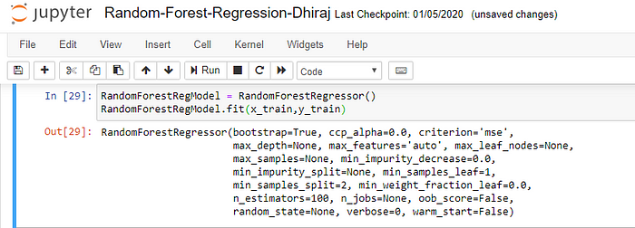
We’re going to use x_train and y_train, obtained above, to train our random forest regression model. We’re using the fit method and passing the parameters as shown below.
Note that the output of this cell is describing a large number of parameters like criteria, max depth, etc. for the model. All these parameters are configurable, and you’re free to tune them to match your requirements.

Prediction
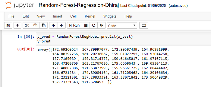
Once the model is trained, it’s ready to make predictions. We can use the predict method on the model and pass x_test as a parameter to get the output as y_pred.
Notice that the prediction output is an array of real numbers corresponding to the input array.

Model Evaluation
Finally, we need to check to see how well our model is performing on the test data. For this, we evaluate our model by finding the root mean squared error produced by the model.
Mean squared error is a built in function, and we are using NumPy’s square root function (np.sqrt) on top of it to find the root mean squared error value.

End notes
In this article, we discussed how to implement linear regression using a random forest algorithm. We also looked at how to pre-process and split the data into features as variable x and labels as variable y.
After that, we trained our model and then used it to run predictions. You can find the data used here.


