Getting Started with Natural Language Processing: US Airline Sentiment Analysis
Sections
- Introduction to NLP
- Dataset Exploration
- NLP Processing
- Training
- Hyperparameter Optimization
- Resources for Future Learning
Introduction to NLP
Natural Language Processing (NLP) is a subfield of machine learning concerned with processing and analyzing natural language data, usually in the form of text or audio. Some common challenges within NLP include speech recognition, text generation, and sentiment analysis, while some high-profile products deploying NLP models include Apple’s Siri, Amazon’s Alexa, and many of the chatbots one might interact with online.
To get started with NLP and introduce some of the core concepts in the field, we’re going to build a model that tries to predict the sentiment (positive, neutral, or negative) of tweets relating to US Airlines, using the popular Twitter US Airline Sentiment dataset.
Code snippets will be included in this post, but for fully reproducible notebooks and scripts, view all of the notebooks and scripts associated with this project on its Comet project page.
Dataset Exploration
Let’s start by importing some libraries. Make sure to install Comet for experiment management, visualizations, code tracking and hyperparameter optimization.
# Comet
from comet_ml import Experiment
A few standard packages: pandas, numpy, matplotlib, etc.
# Standard packages
import os
import pickle
import numpy as np
import pandas as pd
import matplotlib.pyplot as plt
Nltk for natural language processing functions:
# nltk
import nltk
from nltk.tokenize import sent_tokenize, word_tokenize
from nltk.corpus import stopwords
from nltk.stem.snowball import SnowballStemmer
Sklearn and keras for machine learning models:
# sklearn for preprocessing and machine learning models
from sklearn.model_selection import train_test_split
from sklearn.ensemble import GradientBoostingClassifier
from sklearn.metrics import accuracy_score
from sklearn.utils import shuffle
from sklearn.preprocessing import OneHotEncoder
from sklearn.feature_extraction.text import TfidfVectorizer

# Keras for neural networks
from keras.models import Sequential
from keras.layers import Dense, Dropout, BatchNormalization, Flatten
from keras.layers.embeddings import Embedding
from keras.preprocessing import sequence
from keras.utils import to_categorical
from keras.callbacks import EarlyStopping
Now we’ll load the data:
raw_df = pd.read_csv('twitter-airline-sentiment/Tweets.csv')Let’s check the shape of the dataframe:
raw_df.shape()
>>> (14640, 15)
So we’ve got 14,640 samples (tweets), each with 15 features. Let’s take a look at what features this dataset contains.
raw_df.columns'tweet_id' , 'airline_sentiment' , 'airline_sentiment_confidence' , 'negativereason' , 'negativereason_confidence' , 'airline' , 'airline_sentiment_gold' , 'name' , 'negativereason_gold' , 'retweet_count' , 'text' , 'tweet_coord' , 'tweet_created' , 'tweet_location' , 'user_timezone'
Let’s also take a look at airline sentiment for each airline (code can be found on Comet):
# Create a Comet experiment to start tracking our work
experiment = Experiment(
    api_key='<HIDDEN>',
    project_name='nlp-airline',
    workspace='demo')
experiment.add_tag('plotting')
airlines= ['US Airways',
           'United',
           'American',
           'Southwest',
           'Delta',
           'Virgin America']
for i in airlines:
     indices = airlines.index(i)
     new_df=raw_df[raw_df['airline']==i]
     count=new_df['airline_sentiment'].value_counts()
     experiment.log_metric('{} negative'.format(i), count[0])
     experiment.log_metric('{} neutral'.format(i), count[1])
     experiment.log_metric('{} positive'.format(i), count[2])
experiment.end()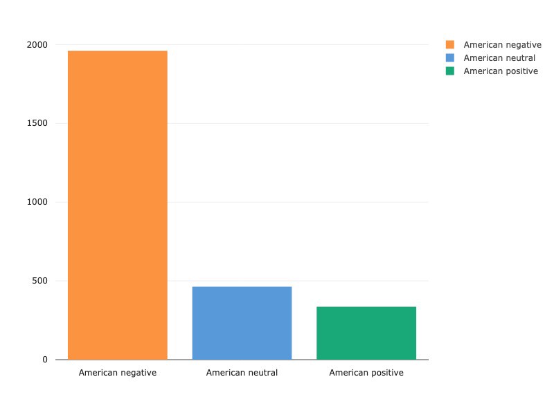
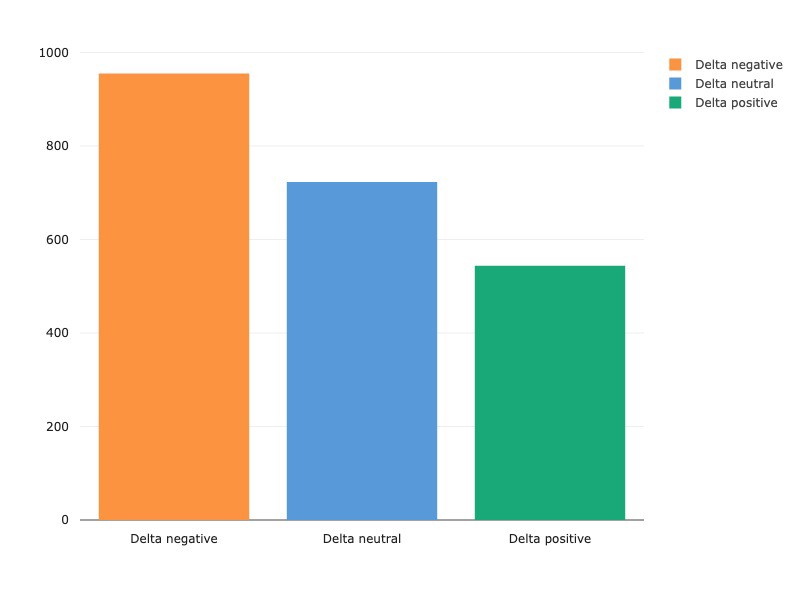
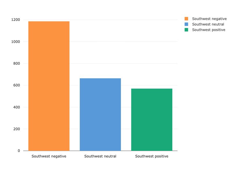
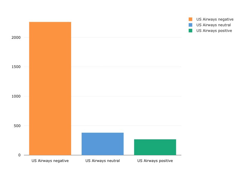
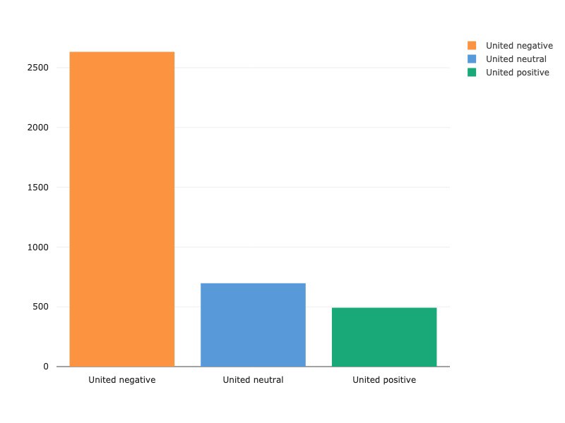
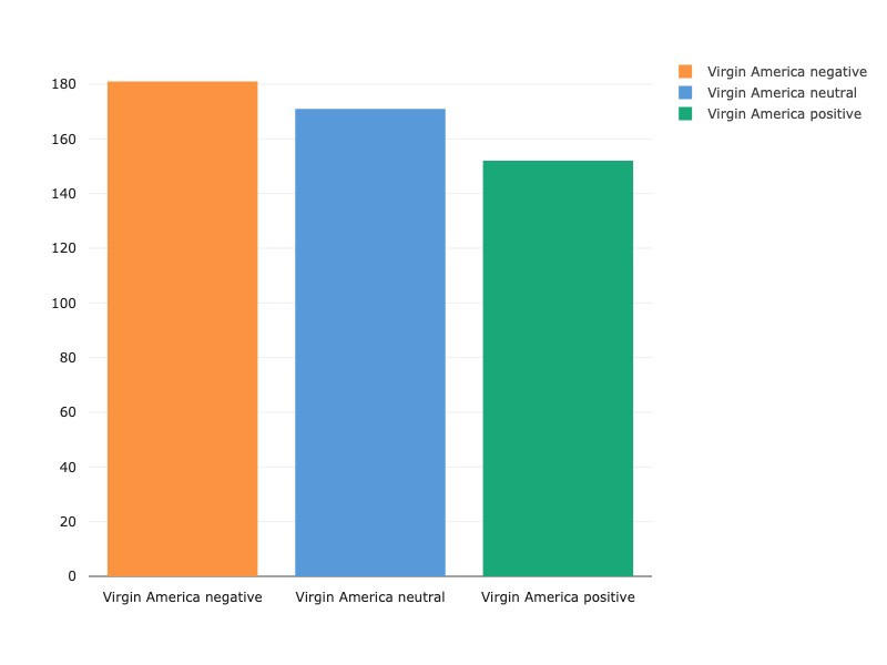
Every airline has more negative tweets than either neutral or positive tweets, with Virgin America receiving the most balanced spread of positive, neutral and negative of all the US airlines. While we’re going to focus on NLP-specific analysis in this write-up, there are excellent sources of further feature-engineering and exploratory data analysis. Kaggle kernels here and here are particularly instructive in analyzing features such as audience and tweet length as related to sentiment.
Let’s create a new dataframe with only tweet_id , text , and airline_sentiment features.
df = raw_df[['tweet_id', 'text', 'airline_sentiment']]And now let’s take a look at a few of the tweets themselves. What’s the data look like?
df['text'][1]

> "@VirginAmerica plus you've added commercials to the experience... tacky."

df['text'][750]

> "@united you are offering us 8 rooms for 32 people #FAIL"

df['text'][5800]

> "@SouthwestAir Your #Android Wi-Fi experience is terrible! $8 is a ripoff! I can't get to @NASCAR or MRN for @DISupdates #BudweiserDuels"
Next, we’re going to conduct a few standard NLP preprocessing techniques to get our dataset ready for training.
NLP Processing
For the purposes of constructing NLP models, one must conduct some basic steps of text preprocessing in order to transfer text from human language to a machine readable format for further processing. Here we will cover some of the standard practices: tokenization, stopword removal, and stemming. You can consult this post to learn about additional text preprocessing techniques.
Tokenization
Given a character sequence and a defined document unit, tokenization is the task of chopping it up into discrete pieces called tokens. In the process of chopping up text, tokenization also commonly involves throwing away certain characters, such as punctuation.

It is simple (and often useful) to think of tokens simply as words, but to fine tune your understanding of the specific terminology of NLP tokenization, the Stanford NLP group’s overview is quite useful.
The NLTK library has a built-in tokenizer we will use to tokenize the US Airline Tweets.
from nltk.tokenize import word_tokenize
def tokenize(sentence):
    tokenized_sentence = word_tokenize(sentence)
    return tokenized_sentence
Stopword Removal
Sometimes, common words that may be of little value in determining the semantic quality of a document are excluded entirely from the vocabulary. These are called stop words. A general strategy for determining a list of stop words is to sort the terms by collection frequency (total number of times each term appears in the document) and then to filter out the most frequent terms as a stop list — hand-filtered by semantic content.

NLTK has a standard stopword list we will adopt here.
from nltk.corpus import stopwords
class PreProcessor:
    def __init__(self, df, column_name):
        self.stopwords = set(stopwords.words('english'))
    def remove_stopwords(self, sentence):
        filtered_sentence = []
        for w in sentence:
            if ((w not in self.stopwords) and
                (len(w) > 1) and
                (w[:2] != '//') and
                (w != 'https')):
                filtered_sentence.append(w)
        return filtered_sentence
Stemming
For grammatical purposes, documents use different forms of a word (look, looks, looking, looked) that in many situations have very similar semantic qualities. Stemming is a rough process by which variants or related forms of a word are reduced (stemmed) to a common base form. As stemming is a removal of prefixed or suffixed letters from a word, the output may or may not be a word belonging to the language corpus. Lemmatization is a more precise process by which words are properly reduced to the base word from which they came.
Examples:
Stemming: car, cars, car’s, cars’ become car
Lemmatization: am, are is become be
Stemmed and Lemmatized Sentence: ‘the boy’s cars are different colors’ become ‘the boy car is differ color’
The most common algorithm for stemming English text is [Porter’s algorithm](TO DO). Snowball, a language for stemming algorithms, was developed by Porter in 2001 and is the basis for the NLTK implementation of its SnowballStemmer, which we will use here.
from nltk.stem.snowball import SnowballStemmer
class PreProcessor:

    def __init__(self, df, column_name):
        self.stemmer = SnowballStemmer('english')
    def stem(self, sentence):
        return [self.stemmer.stem(word) for word in sentence]
Code for these preprocessing steps can be found on Comet.
Next we’ll create a PreProcessor object, containing methods for each of these steps, and run it on the text column of our data frame to tokenize, stem and remove stopwords from the tweets.
preprocessor = PreProcessor(df, 'text')
df['cleaned text'] = preprocessor.full_preprocess()
And now we’ll split our data into training, validation and test sets.
df = shuffle(df, random_state=seed)

# Keep 1000 samples of the data as test set

test_set = df[:1000]

# Get training and validation data

X_train, X_val, y_train, y_val = train_test_split(df['cleaned_text'][1000:], df['airline_sentiment'][1000:], test_size=0.2, random_state=seed)

# Get sentiment labels for test set

y_test = test_set['airline_sentiment']
Now that we’ve split our data into train, validation and test sets, we’ll TF-IDF vectorize them
TF-IDF Vectorization
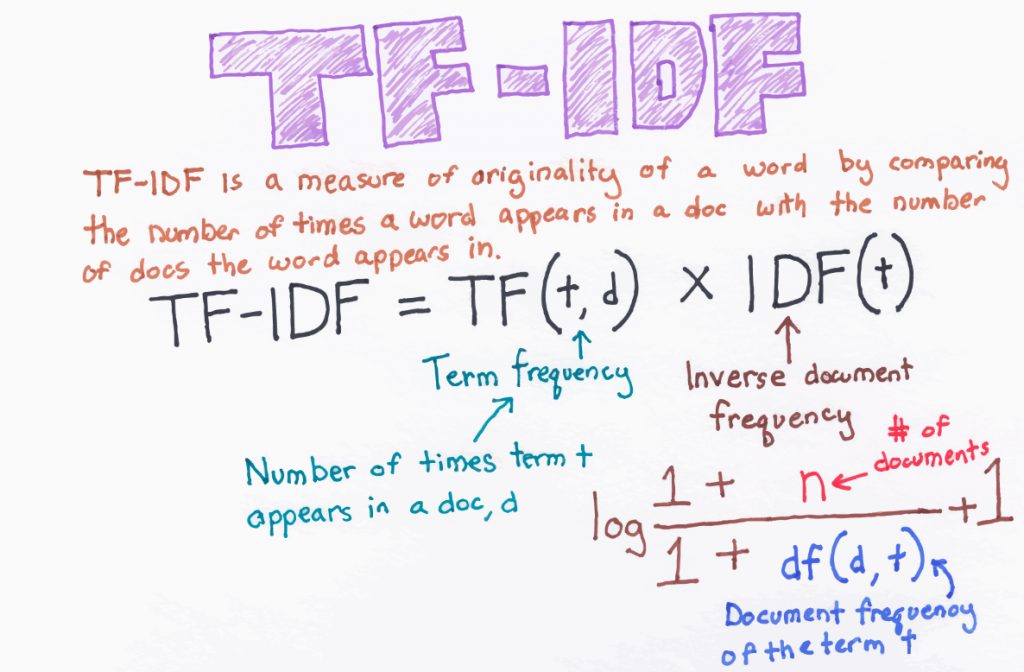
TFIDF, or term frequency — inverse document frequency, is a numerical statistic that reflects how important a word is to a document in a collection or corpus. It is often used to produce weights associated with words that can be useful in searches of information retrieval or text mining. The tf-idf value of a word increases proportionally to the number of times a word appears in a document, and is offset by the number of documents in the corpus that contain that word. This offset helps adjust for the fact that some words appear more frequently in general (think of how stopwords like ‘a’, ‘the’, ‘to’ might have incredibly high tf-idf values if not for offsetting).
We will use scikit-learn’s implementation of TfidfVectorizer, which converts a collection of raw documents (our twitter dataset) into a matrix of TF-IDF features.
vectorizer = TfidVectorizer()
X_train = vectorizer.fit_transform(X_train)
X_val = vectorizer.transform(X_val)
X_test = vectorizer.transform(test_set['cleaned_text'])
Training
We are ready to start training our model. The first thing we’ll do is create a Comet experiment object:
experiment = Experiment(api_key='your-personal-key', project_name='nlp-airline', workspace='demo')
Next, we’ll build a Light Gradient-Boosting classifier (LGBM), an XGBoost classifier, and a relatively straightforward neural network with keras and compare how each of these models performs. Oftentimes it’s hard to tell which architecture will perform best without testing them out. Comet’s project-level view helps make it easy to compare how different experiments are performing and let you easily move from model selection to model tuning.
LGBM
# sklearn's Gradient Boosting Classifier (GBM)

gbm = GradientBoostingClassifier(n_estimators=200, max_depth=6, random_state=seed)

gbm.fit(X_train, y_train)

# Check results

train_pred = gbm.predict(X_train)

val_pred = gbm.predict(X_val)

val_accuracy = round(accuracy_score(y_val,val_pred), 4)

train_accuracy = round(accuracy_score(y_train, train_pred), 4)

# log to comet

experiment.log_metric('val_acc', val_accuracy)

experiment.log_metric('Accuracy', train_accuracy)
XGBOOST
xgb_params = {'objective' : 'multi:softmax',
    'eval_metric' : 'mlogloss',
    'eta' : 0.1,
    'max_depth' : 6,
    'num_class' : 3,
    'lambda' : 0.8,
    'estimators' : 200,
    'seed' : seed
}

target_train = y_train.astype('category').cat.codes

target_val = y_val.astype('category').cat.codes

# Transform data into a matrix so that we can use XGBoost

d_train = xgb.DMatrix(X_train, label = target_train)

d_val = xgb.DMatrix(X_val, label = target_val)

# Fit XGBoost

watchlist = [(d_train, 'train'), (d_val, 'validation')]

bst = xgb.train(xgb_params, d_train, 400, watchlist,

early_stopping_rounds = 50, verbose_eval = 0)

# Check results for XGBoost

train_pred = bst.predict(d_train)

val_pred = bst.predict(d_val)

experiment.log_metric('val_acc', round(accuracy_score(target_val, val_pred)*100, 4))

experiment.log_metric('Accuracy', round(accuracy_score(target_train, train_pred)*100, 4))
Neural Net
# Generator so we can easily feed batches of data to the neural network

def batch_generator(X, y, batch_size, shuffle):
    number_of_batches = X.shape[0]/batch_size
    counter = 0
    sample_index = np.arange(X.shape[0])

    if shuffle:
        np.random.shuffle(sample_index)
    while True:
        batch_index = sample_index[batch_size*counter:batch_size*(counter+1)]
        X_batch = X[batch_index,:].toarray()
        y_batch = y[batch_index]
        counter += 1

        yield X_batch, y_batch
        if (counter == number_of_batches):
            if shuffle:
                np.random.shuffle(sample_index)
            counter = 0

# Initialize sklearn's one-hot encoder class

onehot_encoder = OneHotEncoder(sparse=False)
integer_encoded_train = np.array(y_train).reshape(len(y_train), 1)
onehot_encoded_train = onehot_encoder.fit_transform(integer_encoded_train)
integer_encoded_val = np.array(y_val).reshape(len(y_val), 1)
onehot_encoded_val = onehot_encoder.fit_transform(integer_encoded_val)
experiment.add_tag('NN')

# Neural network architecture

initializer = keras.initializers.he_normal(seed=seed)
activation = keras.activations.elu
optimizer = keras.optimizers.Adam(lr=0.0002, beta_1=0.9, beta_2=0.999, epsilon=1e-8)
es = EarlyStopping(monitor='val_acc', mode='max', verbose=1, patience=4)

# Build model architecture

model = Sequential()
model.add(Dense(20, activation=activation, kernel_initializer=initializer, input_dim=X_train.shape[1]))
model.add(Dropout(0.5))
model.add(Dense(3, activation='softmax', kernel_initializer=initializer))
model.compile(optimizer=optimizer, loss='binary_crossentropy', metrics=['accuracy'])

# Hyperparameters

epochs = 15
batch_size = 32

# Fit the model using the batch_generator

hist = model.fit_generator(generator=batch_generator(X_train, onehot_encoded_train, batch_size=batch_size, shuffle=True), epochs=epochs, validation_data=(X_val, onehot_encoded_val), steps_per_epoch=X_train.shape[0]/batch_size, callbacks=[es])
Comparing our models using Comet’s project view, we can see that our Neural Network models are outperforming the XGBoost and LGBM experiments by a considerable margin.
Let’s select the neural net architecture for now and fine tune it. Note, since we’ve stored all of our experiments — including the XGBoost and LGBM runs we’re not going to use right now — if we decide we’d like to revisit those architectures in the future, all we’ll have to do is view those experiments in the Comet project page and we’ll be able to reproduce them instantly.
Hyperparameter Optimization
Now that we’ve selected our architecture from an initial search of XGBoost, LGBM and a simple keras implementation of a neural network, we’ll need to conduct a hyperparameter optimization to fine-tune our model. Hyperparameter optimization can be an incredibly difficult, computationally expensive, and slow process for complicating modeling tasks. Comet has built an optimization service that can conduct this search for you. Simply pass in the algorithm you’d like to sweep the hyperparameter space with, hyperparameters and ranges to search, and a metric to minimize or maximize, and Comet can handle this part of your modeling process for you.
from comet_ml import Optimizer
config = {
    "algorithm": "bayes",
    "parameters": {
        "batch_size": {"type": "integer", "min": 16, "max": 128},
        "dropout": {"type": "float", "min": 0.1, "max": 0.5},
        "lr": {"type": "float", "min": 0.0001, "max": 0.001},
    },
    "spec": {
        "metric": "loss",
        "objective": "minimize",
    },
}

opt = Optimizer(config, api_key="<HIDDEN>", project_name="nlp-airline", workspace="demo")

for experiment in opt.get_experiments():
    experiment.add_tag('LR-Optimizer')

    # Neural network architecture

    initializer = keras.initializers.he_normal(seed=seed)
    activation = keras.activations.elu
    optimizer = keras.optimizers.Adam(
         lr=experiment.get_parameter("lr"),
         beta_1=0.99,
         beta_2=0.999,
         epsilon=1e-8)

    es = EarlyStopping(monitor='val_acc',
                       mode='max',
                       verbose=1,
                       patience=4)

    batch_size = experiment.get_parameter("batch_size")

    # Build model architecture

    model = Sequential(# Build model like above)
    score = model.evaluate(X_test, onehot_encoded_val, verbose=0)
    logging.info("Score %s", score)
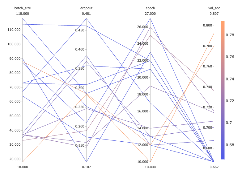
After running our optimization, it is straightforward to select the hyperparameter configuration that yielded the highest accuracy, lowest loss, or whatever performance you were seeking to optimize. Here we keep the optimization problem rather simple: we only search epoch, batch_size, and dropout. The parallel coordinates chart shown below, another native Comet feature, provides a useful visualization of the underlying hyperparameter space our optimizer has traversed:
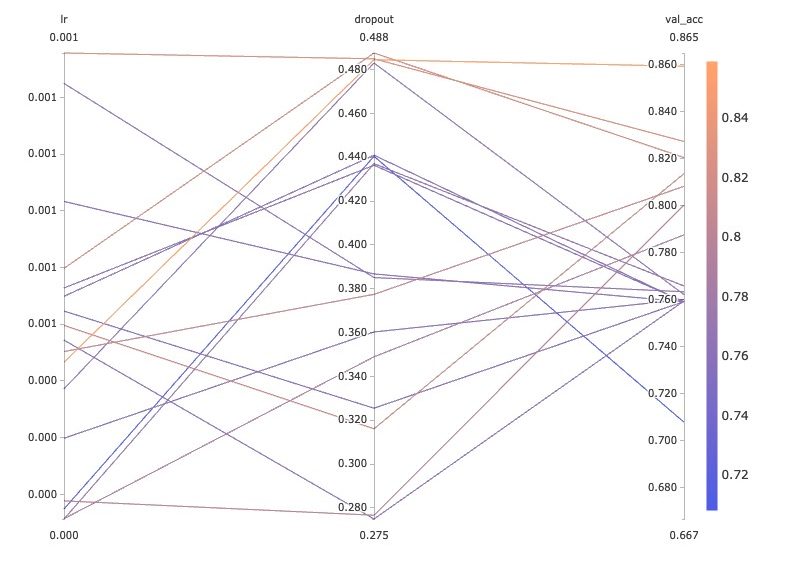
Let’s run another optimization sweep, this time including a range of learning rates to test.
And again we get a view into the regions of the underlying hyperparameter space that are yielding higher values. val_acc
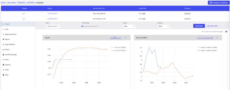
Say now we’d like to compare the performance of two of our better models to keep fine-tuning. Simply select two experiments from your list and click the Diff button and Comet will allow you to visually inspect every code and hyperparameter change, as well as side-by-side visualizations of both experiments.
From here you can continue your model building. Fine tune one of the models we’ve pulled out of the architecture comparison and parameter optimization sweeps, or go back to the start and compare new architectures against our baseline models. All of your work is saved in your Comet project space.
Resources for Future Learning
For additional learning resources in NLP, check out fastai’s new NLP course or this blog post published by Hugging Face that covers some of the best recent papers and trends in NLP. MonkeyLearn has also published a nice article covering sentiment analysis.
