Monitoring Your Time Series Model in Comet
In this tutorial, we will go through steps on how to use Comet to monitor our time-series forecasting model. We will carry out some EDA on our dataset, and then we will log the visualizations onto the Comet experimentation website or platform. Without further ado, let’s begin.
Time Series Models
Time series models are a type of statistical model that are used to analyze and make predictions about data that is collected over time. These models are commonly used in fields such as finance, economics, and weather forecasting.
Some examples of real-life applications of time series models include:
- Forecasting stock prices: Time series models can be used to analyze historical stock prices and make predictions about future prices. This can be useful for investors looking to make informed decisions about purchasing or selling stocks.
- Predicting energy consumption: Time series models can be used to analyze historical energy consumption data and make predictions about future energy demand. This can be useful for utility companies looking to plan for future energy needs.
- Analyzing and forecasting weather patterns: Time series models can be used to analyze historical weather data and make predictions about future weather patterns. This can be useful for weather forecasters and farmers looking to plan for future weather conditions.
- Predictive maintenance: Time series models can be used to predict when equipment is likely to malfunction and schedule maintenance accordingly. This can help reduce downtime and increase efficiency in industries such as manufacturing, transportation, and logistics.
- Time series models can be used in the field of econometrics to analyze and make predictions about economic indicators such as GDP, inflation, and unemployment.
Overall, Time series models are a useful tool that can be used in various industries to evaluate and forecast data gathered over time, assisting businesses in making better decisions and optimizing performance.
Understanding Model Monitoring
Model monitoring is the process of continuously monitoring the performance of a machine-learning model over time. In the context of time series, model monitoring is particularly important as time series data can be highly dynamic because change is definite over time in ways that can impact the accuracy of the model.
For time series data, model monitoring typically involves tracking a set of performance metrics over time to detect any changes or anomalies in the data that may impact the model’s accuracy. These performance metrics may include accuracy, precision, recall, F1 score, and root mean squared error (RMSE), among others.
There are several techniques used for model monitoring with time series data, including:
- Data Drift Detection: This involves monitoring the distribution of the input data over time to detect any changes that may impact the model’s performance.
- Model Performance Monitoring: This involves tracking the performance metrics of the model over time and comparing them to a set of predefined thresholds to detect any degradation in performance.
- Model Retraining: Regular retraining of the model on updated data can help to ensure that the model remains up-to-date and accurate.
- Model Ensemble: Using an ensemble of models can help to detect changes in the data as the outputs of multiple models can be combined to produce a more robust prediction.
It is not necessary to stack all of the techniques mentioned above, and the choice of which technique(s) to use would be determined by the specific requirements of the problem. Model performance monitoring, for example, may suffice if the data is relatively stable and changes occur gradually. However, if the data is highly dynamic and prone to abrupt shifts, data drift detection or model ensemble may be preferable.
Overall, model monitoring is an important aspect of deploying and maintaining machine learning models, especially for time series data where the dynamics of the data can change over time. By continuously monitoring the performance of the model, it is possible to detect and address any issues that may arise and ensure the model remains accurate and reliable.
Comet
Comet is a platform for experimentation that enables you to monitor your machine-learning experiments. Comet has another noteworthy feature: it allows us to conduct exploratory data analysis. We can accomplish our EDA objectives thanks to Comet’s integration with well-known Python visualization frameworks. You can learn more about Comet here.
Prerequisites
You should install the Comet library on your computer if you don’t already have it there by using either of the following lines at the command prompt. Note that if you are installing packages directly into a Colab notebook, or any environment that uses virtual machines, you’ll likely want to use pip.
pip install comet_ml
— or —
conda install -c comet_ml
Have you tried Comet? Sign up for free and easily track experiments, manage models in production, and visualize your model performance.
About The Data
The dataset consists of the sales of cars and the date, year, and month the sales were made. Here is the link to the dataset.
Getting Started
The first step involves loading Comet into our code editor:
from comet_ml import experiment
We then load all the necessary libraries:
import numpy as np
import pandas as pd
import seaborn as sns
import matplotlib.pyplot as plt;
from statsmodels.tsa.seasonal import seasonal_decompose
from tensorflow.keras.models import Sequential
from tensorflow.keras.layers import Dense, InputLayer
import warnings
warnings.filterwarnings('ignore')
We then load our dataset so we can perform some EDA:
Car_sales = pd.read_csv('/content/sales-cars.csv')
After loading the dataset we then begin some EDA on our dataset.
The below method .head() is used to fetch the initial rows of a DataFrame, where the number within the parentheses determines the number of rows to retrieve from the main dataset.
For instance, as we execute Car_sales.head(10) below, it would then extract the first ten rows of the Car_sales DataFrame. This process gives a fast evaluation of a small set of data, providing insight into its arrangement and details.
Car_sales.head(10)

Car_sales.tail()
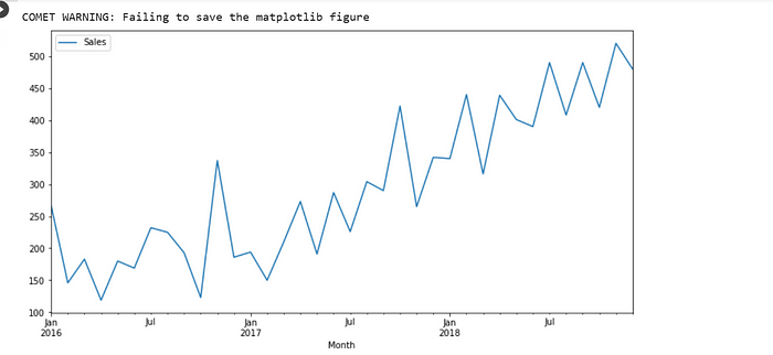
We then plot a figure to show the sales of cars per month.
fig1 =Car_sales.plot(figsize=(12,6));
experiment.log_figure(figure_name="Sales vs Month", figure=fig1)
plt.show()

From the graph above we can see that the sales of cars increased drastically over the months. Most particularly in July of each Year.
Moving on we then check the seasonal sales of cars using the seasonal forecast code.
fig2 = plt.figure(figsize=(15,2))
results = seasonal_decompose(Car_sales['Sales'])
experiment.log_figure(figure_name= "Seasonal Forcast", figure=fig2)
results.plot();

We then divide the dataset into TEST and TRAIN
train = Car_sales[:-6]
test = Car_sales[-6:]
After dividing the dataset we then perform some EDA on the Train dataset.
To acquire a deeper knowledge of the dataset and undertake exploratory data analysis, the train.head() function is frequently used in conjunction with other methods such as train.info() and train.describe(). By looking at the first few rows of the dataset, you may get a feel of how the data is distributed, detect any missing or inconsistent values, and start to generate hypotheses about the relationship between variables in the dataset.
train.head()

We also perform EDA on the test dataset.
test.head()

def generate_lag(Car_sales, n):
    X, y = [], []
    for i in range(len(Car_sales) - n):
        X.append(Car_sales[i:i+n])
        y.append(Car_sales[n+i])

    return np.array(X), np.array(y), np.array(y[-n:]).reshape(1,n)
The preceding code defines the function “generate lag,” which accepts two arguments: “Car sales” (a list or array of numerical data) and “n.” (an integer). The function provides lag data for time series analysis by producing input-output pairs. As the output, it generates “n”-length sequences of “Car sales” and their associated next values.
Three NumPy arrays are returned by the function:
“X” is a two-dimensional array in which each row contains a “n”-length series of “Car sales” data.
“y”: a 1D array with each member reflecting the next value in the time series following the corresponding sequence in “X.”
The previous “n” values of “y” were rearranged into a 1-row, “n”-column array. This is the most current data in the time series that the function can forecast.
def forecast_function(model, last_batch, n):
    in_value = last_batch.copy()
    preds = []
    for i in range(n):
        p = model.predi ct(in_value)
        preds.append(p.ravel())
        in_value = np.append(in_value, p)[1:].reshape(last_batch.shape)
    return np.array(preds).ravel()
The code specifies the “forecast function” function, which accepts three arguments: “model” (a trained predictive model), “last batch” (a NumPy array containing the latest “n” values of a time series), and “n” (an integer representing the number of time steps to predict into the future).
Using the “model” supplied as input, the function creates “n” predictions for a time series. It begins by copying the array “last batch” into a variable named “in value.” It then begins an iterative loop that repeats “n” times. It utilizes the “model” to make a forecast for the next value in the time series in each iteration, using the most recent “n” values (originally “last batch”) as input. The predicted value is saved in the “preds” list.
The code then modifies the “in value” variable by attaching the predicted value to the end and removing the initial value, essentially shifting the array to the right by one-time step. The new “in value” is reshaped to match the original “last batch” form.
The function returns the predicted values in a 1D NumPy array named “preds” when the loop is done.
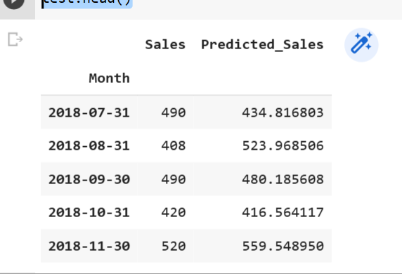
test['Predicted_Sales']=pred
The above line of code adds a new column to the test dataframe and then assigns it to ‘pred.’
Let’s view the new predicted column:
test.head()

We can see that the predicted sales are higher than the original sales. Let’s visualize the predicted sales vs. normal sales.
fig3 = plt.figure(figsize=(15,2))
experiment.log_figure(figure_name= "Sales vs preditced sales", figure=fig3)
test.plot()

The visuals confirm that the predicted sales are higher in most cases compared to the actual sales.
We need to determine the percentage error of the predicted sales so the code below checks for the percentage error.
def error_function(Car_sales,column_1,column_2):
    data = Car_sales.copy()
    my_list = []
    for i in range(len(data)):
        x = (data[column_2][i]*100)/data[column_1][i]
        if x >= 100:
            error = x-100
            #data['error_percentage'][i] = error
            my_list.append(error)
        else:
            error = 100-x
            my_list.append(error)
            #data['error_percentage'][i] = error
    data['error_percentage'] = my_list
    return data
The code specifies the “error function” function, which accepts three arguments: “Car sales” (a pandas DataFrame), “column 1” (a string representing the label of one column in “Car sales”), and “column 2” (a string representing the label of another column in “Car sales”).
For each entry in the “Car sales” DataFrame, the function computes the percentage error between the two columns defined by “column 1” and “column 2.” It begins by creating a “data” DataFrame replica of the “Car sales” DataFrame.
It then begins a loop that iterates through each entry in the “data” array. It computes the % difference between the values in “column 1” and “column 2” for each row. If the % difference exceeds 100, the error is calculated as the difference between the percentage difference and 100. If the % difference is less than 100, the error is equal to 100 minus the percentage difference. Each error value is appended to a list named “my list” by the function.
After the loop is ended, the method adds a new column to the “data” DataFrame named “error percentage”, which includes the percentage errors saved in “my list.”
The function returns the “data” DataFrame with the new column “error percentage” added.
column_1 = 'Sales'
column_2 = 'Predicted_Sales'
Car_sales_new = error_function(test,column_1,column_2)
Car_sales_new

We then view our experiment on Comet:
Comet’s ability to automatically log and track experiment metadata, such as hyperparameters, metrics, and model artifacts, is one of the key ways it simplifies model monitoring. Data scientists can easily compare the performance of different models and hyperparameter configurations and monitor the training process in real time by tracking experiments with Comet. This enables them to quickly identify potential issues, such as over- or under-fitting, and adjust their models as needed.
Comet also includes a set of visualization tools to help you explore and interpret experimental results. Users can, for example, view learning curves to track model performance over time or scatter plots and heatmaps to compare the behavior of different models across a variety of metrics.
Comet also has the ability to connect with popular machine learning frameworks which include: TensorFlow and PyTorch. This implies that users may log experiments and metrics straight from their code, with no further setup or configuration required.
Conclusion
In conclusion, model monitoring is a critical step in the machine learning pipeline, and Comet ML is an excellent tool for tracking and visualizing model performance.
Through Comet, data scientists can monitor their models in real-time, identify problems early, and make quick decisions to improve model accuracy. The platform enables users to view and analyze model performance metrics, compare different models, and visualize model training and evaluation results.
Comet also allows users to collaborate and share experiments with team members, which is particularly beneficial for distributed teams. Furthermore, the platform integrates with many popular machine learning libraries and frameworks, making it easy to incorporate into existing workflows.
Overall, Comet provides a comprehensive and user-friendly platform for model monitoring that can help data scientists to optimize their models and make better-informed decisions. You can get the full code here.


