Introduction to Machine Learning Model Evaluation

Machine learning continues to be an increasingly integral component of our lives, whether we’re applying the techniques to research or business problems. Machine learning models ought to be able to give accurate predictions in order to create real value for a given organization.
While training a model is a key step, how the model generalizes on unseen data is an equally important aspect that should be considered in every machine learning pipeline. We need to know whether it actually works and, consequently, if we can trust its predictions. Could the model be merely memorizing the data it is fed with, and therefore unable to make good predictions on future samples, or samples that it hasn’t seen before?
In this article, we explain the techniques used in evaluating how well a machine learning model generalizes to new, previously unseen data. We’ll also illustrate how common model evaluation metrics are implemented for classification and regression problems using Python.
Model Evaluation Techniques
The above issues can be handled by evaluating the performance of a machine learning model, which is an integral component of any data science project. Model evaluation aims to estimate the generalization accuracy of a model on future (unseen/out-of-sample) data.
Methods for evaluating a model’s performance are divided into 2 categories: namely, holdout and Cross-validation. Both methods use a test set (i.e data not seen by the model) to evaluate model performance. It’s not recommended to use the data we used to build the model to evaluate it. This is because our model will simply remember the whole training set, and will therefore always predict the correct label for any point in the training set. This is known as overfitting.
Holdout
The purpose of holdout evaluation is to test a model on different data than it was trained on. This provides an unbiased estimate of learning performance.
In this method, the dataset is randomly divided into three subsets:
- Training set is a subset of the dataset used to build predictive models.
- Validation set is a subset of the dataset used to assess the performance of the model built in the training phase. It provides a test platform for fine-tuning a model’s parameters and selecting the best performing model. Not all modeling algorithms need a validation set.
- Test set, or unseen data, is a subset of the dataset used to assess the likely future performance of a model. If a model fits to the training set much better than it fits the test set, overfitting is probably the cause.
The holdout approach is useful because of its speed, simplicity, and flexibility. However, this technique is often associated with high variability since differences in the training and test dataset can result in meaningful differences in the estimate of accuracy.
Cross-Validation
Cross-validation is a technique that involves partitioning the original observation dataset into a training set, used to train the model, and an independent set used to evaluate the analysis.
The most common cross-validation technique is k-fold cross-validation, where the original dataset is partitioned into k equal size subsamples, called folds. The k is a user-specified number, usually with 5 or 10 as its preferred value. This is repeated k times, such that each time, one of the k subsets is used as the test set/validation set and the other k-1 subsets are put together to form a training set. The error estimation is averaged over all k trials to get the total effectiveness of our model.
For instance, when performing five-fold cross-validation, the data is first partitioned into 5 parts of (approximately) equal size. A sequence of models is trained. The first model is trained using the first fold as the test set, and the remaining folds are used as the training set. This is repeated for each of these 5 splits of the data and the estimation of accuracy is averaged over all 5 trials to get the total effectiveness of our model.
As can be seen, every data point gets to be in a test set exactly once and gets to be in a training set k-1 times. This significantly reduces bias, as we’re using most of the data for fitting, and it also significantly reduces variance, as most of the data is also being used in the test set. Interchanging the training and test sets also adds to the effectiveness of this method.
Model Evaluation Metrics
Model evaluation metrics are required to quantify model performance. The choice of evaluation metrics depends on a given machine learning task (such as classification, regression, ranking, clustering, topic modeling, among others). Some metrics, such as precision-recall, are useful for multiple tasks. Supervised learning tasks such as classification and regression constitutes a majority of machine learning applications. In this article, we focus on metrics for these two supervised learning models.
Classification Metrics
In this section we will review some of the metrics used in classification problems, namely:
- Classification Accuracy
- Confusion matrix
- Logarithmic Loss
- Area under curve (AUC)
- F-Measure
Classification Accuracy
Accuracy is a common evaluation metric for classification problems. It’s the number of correct predictions made as a ratio of all predictions made. We use sklearn module to compute the accuracy of a classification task, as shown below:
#import modules
import warnings
import pandas as pd
import numpy as np
from sklearn import model_selection
from sklearn.linear_model import LogisticRegression
from sklearn import datasets
from sklearn.metrics import accuracy_score
#ignore warnings
warnings.filterwarnings('ignore')
# Load digits dataset
iris = datasets.load_iris()
# # Create feature matrix
X = iris.data
# Create target vector
y = iris.target
#test size
test_size = 0.33
#generate the same set of random numbers
seed = 7
#cross-validation settings
kfold = model_selection.KFold(n_splits=10, random_state=seed)
#Model instance
model = LogisticRegression()
#Evaluate model performance
scoring = 'accuracy'
results = model_selection.cross_val_score(model, X, y, cv=kfold, scoring=scoring)
print('Accuracy -val set: %.2f%% (%.2f)' % (results.mean()*100, results.std()))

#split data
X_train, X_test, y_train, y_test = model_selection.train_test_split(X, y, test_size=test_size, random_state=seed)
#fit model
model.fit(X_train, y_train)
#accuracy on test set
result = model.score(X_test, y_test)
print("Accuracy - test set: %.2f%%" % (result*100.0))
The classification accuracy is 88% on the validation set.
By using cross-validation, we’d be “testing” our machine learning model in the “training” phase to check for overfitting and to get an idea about how our machine learning model will generalize to independent data (test data set).
Cross-validation techniques can also be used to compare the performance of different machine learning models on the same data set and can also be helpful in selecting the values for a model’s parameters that maximize the accuracy of the model—also known as parameter tuning.
Confusion Matrix
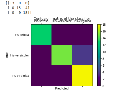
A confusion matrix provides a more detailed breakdown of correct and incorrect classifications for each class. We use the Iris dataset to classify and compute the confusion matrix for the predictions:
#import modules
import warnings
import pandas as pd
from sklearn import model_selection
from sklearn.linear_model import LogisticRegression
from sklearn.metrics import confusion_matrix
import matplotlib.pyplot as plt
%matplotlib inline

#ignore warnings
warnings.filterwarnings('ignore')
# Load digits dataset
url = "http://archive.ics.uci.edu/ml/machine-learning-databases/iris/iris.data"
df = pd.read_csv(url)
# df = df.values
X = df.iloc[:,0:4]
y = df.iloc[:,4]
# print (y.unique())
#test size
test_size = 0.33
#generate the same set of random numbers
seed = 7
#Split data into train and test set.
X_train, X_test, y_train, y_test = model_selection.train_test_split(X, y, test_size=test_size, random_state=seed)
#Train Model
model = LogisticRegression()
model.fit(X_train, y_train)
pred = model.predict(X_test)

#Construct the Confusion Matrix
labels = ['Iris-setosa', 'Iris-versicolor', 'Iris-virginica']
cm = confusion_matrix(y_test, pred, labels)
print(cm)
fig = plt.figure()
ax = fig.add_subplot(111)
cax = ax.matshow(cm)
plt.title('Confusion matrix of the classifier')
fig.colorbar(cax)
ax.set_xticklabels([''] + labels)
ax.set_yticklabels([''] + labels)
plt.xlabel('Predicted')
plt.ylabel('True')
plt.show()

The short explanation of how to interpret a confusion matrix is as follows: The diagonal elements represent the number of points for which the predicted label is equal to the true label, while anything off the diagonal was mislabeled by the classifier. Therefore, the higher the diagonal values of the confusion matrix the better, indicating many correct predictions.
In our case, the classifier predicted all the 13 setosa and 18 virginica plants in the test data perfectly. However, it incorrectly classified 4 of the versicolor plants as virginica.
Logarithmic Loss
Logarithmic loss (logloss) measures the performance of a classification model where the prediction input is a probability value between 0 and 1. Log loss increases as the predicted probability diverges from the actual label. The goal of machine learning models is to minimize this value. As such, smaller logloss is better, with a perfect model having a log loss of 0.
#Classification LogLoss
import warnings
import pandas
from sklearn import model_selection
from sklearn.linear_model import LogisticRegression
from sklearn.metrics import log_loss

warnings.filterwarnings('ignore')
url = "https://raw.githubusercontent.com/jbrownlee/Datasets/master/pima-indians-diabetes.data.csv"
dataframe = pandas.read_csv(url)
dat = dataframe.values
X = dat[:,:-1]
y = dat[:,-1]
seed = 7
#split data
X_train, X_test, y_train, y_test = model_selection.train_test_split(X, y, test_size=test_size, random_state=seed)
model.fit(X_train, y_train)
#predict and compute logloss
pred = model.predict(X_test)
accuracy = log_loss(y_test, pred)
print("Logloss: %.2f" % (accuracy))
Area under Curve (AUC)
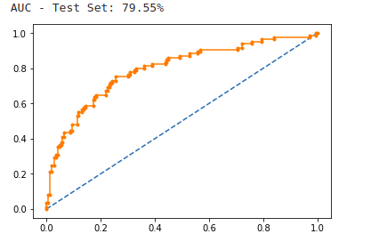
Area under ROC Curve is a performance metric for measuring the ability of a binary classifier to discriminate between positive and negative classes.
#Classification Area under curve
import warnings
import pandas
from sklearn import model_selection
from sklearn.linear_model import LogisticRegression
from sklearn.metrics import roc_auc_score, roc_curve

warnings.filterwarnings('ignore')

url = "https://raw.githubusercontent.com/jbrownlee/Datasets/master/pima-indians-diabetes.data.csv"
dataframe = pandas.read_csv(url)
dat = dataframe.values
X = dat[:,:-1]
y = dat[:,-1]
seed = 7
#split data
X_train, X_test, y_train, y_test = model_selection.train_test_split(X, y, test_size=test_size, random_state=seed)
model.fit(X_train, y_train)

# predict probabilities
probs = model.predict_proba(X_test)
# keep probabilities for the positive outcome only
probs = probs[:, 1]

auc = roc_auc_score(y_test, probs)
print('AUC - Test Set: %.2f%%' % (auc*100))

# calculate roc curve
fpr, tpr, thresholds = roc_curve(y_test, probs)
# plot no skill
plt.plot([0, 1], [0, 1], linestyle='--')
# plot the roc curve for the model
plt.plot(fpr, tpr, marker='.')
# show the plot
plt.show()

In the example above, the AUC is relatively close to 1 and greater than 0.5. A perfect classifier will have the ROC curve go along the Y axis and then along the X axis.
F-Measure
F-measure (also F-score) is a measure of a test’s accuracy that considers both the precision and the recall of the test to compute the score. Precision is the number of correct positive results divided by the total predicted positive observations. Recall, on the other hand, is the number of correct positive results divided by the number of all relevant samples (total actual positives).
import warnings
import pandas
from sklearn import model_selection
from sklearn.linear_model import LogisticRegression
from sklearn.metrics import log_loss
from sklearn.metrics import precision_recall_fscore_support as score, precision_score, recall_score, f1_score

warnings.filterwarnings('ignore')

url = "https://raw.githubusercontent.com/jbrownlee/Datasets/master/pima-indians-diabetes.data.csv"
dataframe = pandas.read_csv(url)
dat = dataframe.values
X = dat[:,:-1]
y = dat[:,-1]
test_size = 0.33
seed = 7

model = LogisticRegression()
#split data
X_train, X_test, y_train, y_test = model_selection.train_test_split(X, y, test_size=test_size, random_state=seed)
model.fit(X_train, y_train)
precision = precision_score(y_test, pred)
print('Precision: %f' % precision)
# recall: tp / (tp + fn)
recall = recall_score(y_test, pred)
print('Recall: %f' % recall)
# f1: tp / (tp + fp + fn)
f1 = f1_score(y_test, pred)
print('F1 score: %f' % f1)
Regression Metrics
In this section we review 2 of the most common metrics for evaluating regression problems namely, Root Mean Squared Error and Mean Absolute Error.
The Mean Absolute Error (or MAE) is the sum of the absolute differences between predictions and actual values. On the other hand, Root Mean Squared Error (RMSE) measures the average magnitude of the error by taking the square root of the average of squared differences between prediction and actual observation.
The Python code snippet below shows how the two regression metrics can be implemented.
import pandas
from sklearn import model_selection
from sklearn.linear_model import LinearRegression
from sklearn.metrics import mean_absolute_error, mean_squared_error
from math import sqrt
url = "https://raw.githubusercontent.com/jbrownlee/Datasets/master/housing.data"
dataframe = pandas.read_csv(url, delim_whitespace=True)
df = dataframe.values
X = df[:,:-1]
y = df[:,-1]
seed = 7
model = LinearRegression()
#split data
X_train, X_test, y_train, y_test = model_selection.train_test_split(X, y, test_size=test_size, random_state=seed)
model.fit(X_train, y_train)
#predict
pred = model.predict(X_test)
print("MAE test score:", mean_absolute_error(y_test, pred))
print("RMSE test score:", sqrt(mean_squared_error(y_test, pred)))
Conclusion
Ideally, the estimated performance of a model tells us how well it performs on unseen data. Making predictions on future data is often the main problem we want to solve. It’s important to understand the context before choosing a metric because each machine learning model tries to solve a problem with a different objective using a different dataset.
This article has attempted to explain the common evaluation metrics for classification and regression machine learning problems, providing short Python snippets to show how they can be implemented.
Discuss this post on Hacker News and Reddit.


