Introducing YOLO-NAS: A New State-of-the-Art for Object Detection
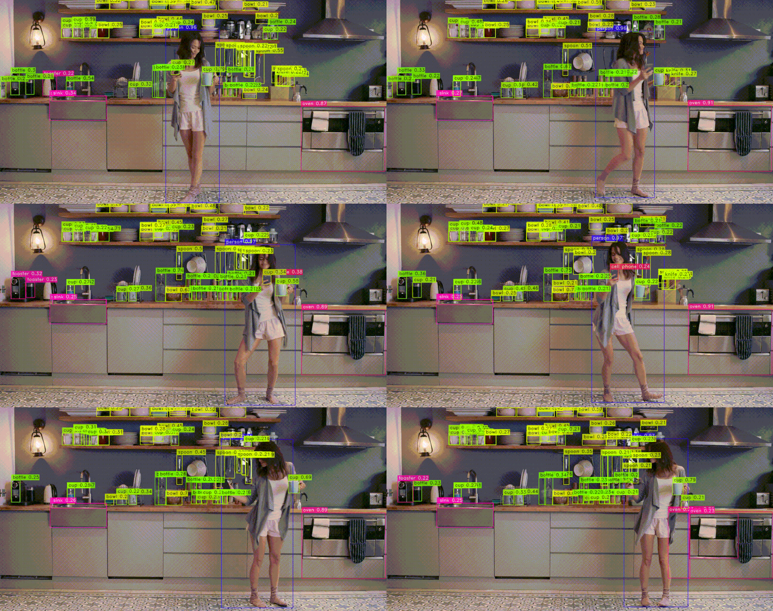
YOLO models are famous for two main reasons:
- Impressive speed and accuracy.
- Ability to detect objects in images quickly and dependably.
The first version of YOLO was introduced in 2016 and changed how object detection was performed by treating object detection as a single regression problem.
It divided images into a grid and simultaneously predicted bounding boxes and class probabilities. Though it was faster than previous object detection methods, YOLOv1 had limitations in detecting small objects and struggled with localization accuracy. Since the first YOLO architecture hit the scene, 15 YOLO-based architectures have been developed, all known for their accuracy, real-time performance, and enabling object detection on edge devices and in the cloud.
But just because we have all these YOLOs doesn’t mean that deep learning for object detection is a dormant area of research.
In the subfield of computer vision, the competition for cutting-edge object detection is fierce.
At Deci, a team of researchers aimed to create a model that would stand out amongst the rest. Their objective was to make revolutionary improvements, just as sprinters aim to shave milliseconds off their times. The team embraced the challenge of pushing the limits of performance, knowing that even small increases in mAP and reduced latency could truly revolutionize the object detection model landscape.
And in the process, a new YOLO architecture was born: 🏎️YOLO-NAS
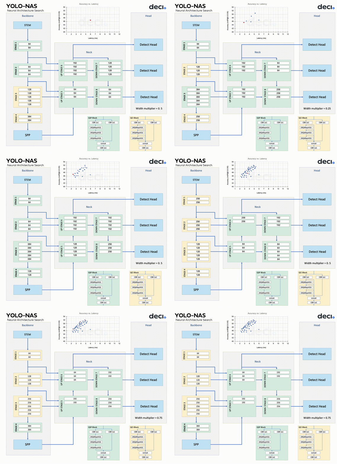
YOLO-NAS is composed of a backbone, neck, and head, mirroring many similar models.
The backbone extracts features from the input image.
YOLO-NAS has a dual-path backbone with dense feature extraction and sparse feature fusion paths. The dense path has multiple convolutional layers with skip connections in dense blocks, while the transition blocks in the sparse path reduce spatial resolution and boost the number of channels. Both paths interconnect via cross-stage partial connections, which enables gradient flow.
Innovation and academia go hand-in-hand. Listen to our own CEO Gideon Mendels chat with the Stanford MLSys Seminar Series team about the future of MLOps and give the Comet platform a try for free!
The neck further enhances the features extracted by the backbone, creating predictions at varied scales.
The YOLO-NAS system utilizes a multi-scale feature pyramid and backbone features to make small, medium, and large predictions. The neck of the system combines upsampling and concatenation to blend features from various levels, thus broadening the receptive field. The head performs final classification and regression tasks.
The YOLO-NAS head consists of two parallel branches.
One is a classification branch, and the other is a regression branch that uses generalized IoU loss. The classification branch predicts the class probability of each anchor box, while the regression branch estimates the bounding box coordinates.
What’s New in 🏎️YOLO-NAS?
✨ YOLO-NAS utilizes cutting-edge methods such as attention mechanisms, quantization aware blocks, and inference time reparametrization, raising the bar for object detection in various industries.
✨ It’s an open-source model with pre-trained weights (for non-commercial research) through Deci’s PyTorch-based computer vision library called SuperGradients.
✨ It’s a foundation model for object detection pretrained on COCO, Objects365, and Roboflow 100, preparing you for success in downstream object detection tasks.
✨ The algorithm for selecting layers in the model quantizes certain parts to minimize loss of information while ensuring a balance between latency and accuracy.
✨ Post-training, the network converts to INT8, enhancing efficiency even further.
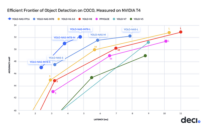
✨ Compared to other top YOLO models, YOLO-NAS (m) model achieves a 50% increase in throughput and a 1 mAP improvement in accuracy on the NVIDIA T4 GPU.
There’s no paper for YOLO-NAS, but a technical blog details the architecture and training procedure.
🫣 Sneak peek: Inference with YOLO-NAS
Before jumping into the section on fine-tuning, I wanted to show you the power of YOLONAS out of the box.
Start by instantiating a pretrained model. YOLONAS comes in three flavors: yolo_nas_s, yolo_nas_m, and yolo_nas_l.
You’ll use yolo_nas_l throughout this tutorial. Because you should always go big or go home.
It’s a good life philosophy.
👨🏽🔧 Install SuperGradients
🚨 Note (for Google Colab): after installation is complete (it will take a few minutes), you’ll need to restart the runtime after installation completion.
This is a known issue that is on our roadmap.
pip install super-gradients==3.1.1
👇🏽Instantiate a pre-trained model
from super_gradients.training import models

yolo_nas_l = models.get("yolo_nas_l", pretrained_weights="coco")
🖼️ Inference on an image
Once the model has been instantiated all you have to do is call the predictmethod.
This method operates on:
✳️ PIL Image
️️✳️ Numpy Image
✳️ A path to an image file
✳️ A path to video file
✳️ A path to folder with images
✳️ URL (Image only)
Note: Predict also has an argument called conf, the threshold for detection. You change this value as you like, for example: model.predict(“path/to/asset”,conf=0.25).
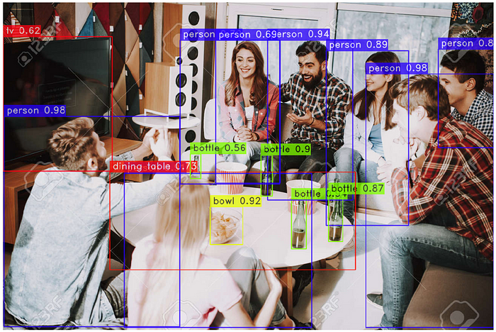
Let’s perform inference on the following image:

url = "https://previews.123rf.com/images/freeograph/freeograph2011/freeograph201100150/158301822-group-of-friends-gathering-around-table-at-home.jpg"
yolo_nas_l.predict(url, conf=0.25).show()
🤷🏽♂️ What’s happening “under the hood”
- Input image gets through the preprocessing pipeline, which includes image resizing, normalization, and permute operation to convert input RGB image to torch tensor.
- Model inference
- Postprocessing of the detection results (Non-maximum suppression, resizing bounding boxes to the size of the original image)
- Visualization of the results (Rendering of bounding boxes on top of the image)
🏋🏽 The Trainer
The first thing you need to define in SuperGradients is the Trainer.
The trainer oversees training, evaluation, saving checkpoints, etc. If you’re interested in seeing the source code for the trainer, you can do so here.
✌🏼 There are two important arguments for the trainer:
1) ckpt_root_dir — this is the directory where results from all your experiments will be saved
2) experiment_name — all checkpoints, logs, and tensorboards will be saved in a directory with the name you specify here.
SuperGradients supports Data Parallel and Distributed Data Parallel.
That’s outside of the scope of this introduction to SuperGradients. But if you’re fortunate enough to have multiple GPUs or want to learn more, you can do so here.
In the code below, you’ll instantiate the trainer with just a single GPU (since that’s what Google Colab provides)
from super_gradients.training import Trainer

CHECKPOINT_DIR = 'checkpoints'
trainer = Trainer(experiment_name='my_first_yolonas_run', ckpt_root_dir=CHECKPOINT_DIR)
💾 Datasets and DataLoaders
SuperGradients is fully compatible with PyTorch Datasets and Dataloaders, so you can use your dataloaders as is.
There are several well-known datasets for object detection, for example:
💽 COCO
💽 Pascal
💽 YOLODarkNet
💽 YOLOv5
SuperGradients provides ready-to-use dataloaders for these datasets. If you’re interested in learning more about working with COCOFormatDetectionDataset and the more general DetectionDataset check out the SuperGradients documentation on this topic.
You can learn more about working with SuperGradients datasets, dataloaders, and configuration files here.
SuperGradients supports several dataset formats. You can learn more about that here.
For this example, you’ll use the U.S. Coins Dataset from RoboFlow with the dataset in YOLOv5 format.
from roboflow import Roboflow
rf = Roboflow(api_key="<your-roboflow-key-here>")
project = rf.workspace("atathamuscoinsdataset").project("u.s.-coins-dataset-a.tatham")
dataset = project.version(5).download("yolov5")
Start by importing the required modules to help you create SuperGradients dataloaders.
from super_gradients.training import dataloaders
from super_gradients.training.dataloaders.dataloaders import coco_detection_yolo_format_train, coco_detection_yolo_format_val
You’ll need to load your dataset parameters into a dictionary, specifically defining:
✳️ Path to the parent directory where your data lives
️️✳️ The child directory names for training, validation, and test (if you have test set) images and labels
✳️ Class names
You pass the values for dataset_params into the dataset_params argument, as shown below.
dataset_params = {
    'data_dir':'/content/U.S.-Coins-Dataset---A.Tatham-5',
    'train_images_dir':'train/images',
    'train_labels_dir':'train/labels',
    'val_images_dir':'valid/images',
    'val_labels_dir':'valid/labels',
    'test_images_dir':'test/images',
    'test_labels_dir':'test/labels',
    'classes': ['Dime', 'Nickel', 'Penny', 'Quarter']
You can also pass PyTorch DataLoaders arguments when instantiating your dataset. Here you’ll set batch_size=16 and num_workers=2.
Repeat this for the validation and testing datasets. Note that for training and testing data, we use coco_detection_yolo_format_val to instantiate the dataloader.
The dataloaders will print warnings when an annotation does not conform to the expected format. This dataset has many such annotations; thus, the warnings will be muted.
from IPython.display import clear_output

train_data = coco_detection_yolo_format_train(
    dataset_params={
        'data_dir': dataset_params['data_dir'],
        'images_dir': dataset_params['train_images_dir'],
        'labels_dir': dataset_params['train_labels_dir'],
        'classes': dataset_params['classes']
    },
    dataloader_params={
        'batch_size':16,
        'num_workers':2
    }
)

val_data = coco_detection_yolo_format_val(
    dataset_params={
        'data_dir': dataset_params['data_dir'],
        'images_dir': dataset_params['val_images_dir'],
        'labels_dir': dataset_params['val_labels_dir'],
        'classes': dataset_params['classes']
    },
    dataloader_params={
        'batch_size':16,
        'num_workers':2
    }
)

test_data = coco_detection_yolo_format_val(
    dataset_params={
        'data_dir': dataset_params['data_dir'],
        'images_dir': dataset_params['test_images_dir'],
        'labels_dir': dataset_params['test_labels_dir'],
        'classes': dataset_params['classes']
    },
    dataloader_params={
        'batch_size':16,
        'num_workers':2
    }
)

clear_output()
👩🏽🦳 Instantiating the model
You saw how to instantiate the model for inference earlier.
Below is how to instantiate the model for finetuning. Note you need to add the num_classes argument here.
Note, for this tutorial, you’re using yolo_nas_l, but SuperGradients has two other flavors of YOLONAS available to you: yolo_nas_s and yolo_nas_m.
from super_gradients.training import models
model = models.get('yolo_nas_l',
                   num_classes=len(dataset_params['classes']),
                   pretrained_weights="coco"
                   )
🎛️ Training parameters
You need to define the training parameters for your training run.
Full details about the training parameters can be found here.
🚨 There are a few mandatory arguments that you must define for training params 🚨
✳️ max_epochs — Max number of training epochs
✳️️️ loss— the loss function you want to use
✳️ optimizer— Optimizer you will be using
✳️ train_metrics_list — Metrics to log during training
✳️ valid_metrics_list — Metrics to log during training
✳️ metric_to_watch — metric which the model checkpoint will be saved according to
You can choose from various optimizers such as Adam, AdamW, SGD, Lion, or RMSProps. If you change the default parameters of these optimizers, you pass them into optimizer_params.
🔕 Note: I’ve enabled silent_mode, so the notebook doesn’t get longer than it already is. You should disable it so you can see what SuperGradients outputs during training.
from super_gradients.training.losses import PPYoloELoss
from super_gradients.training.metrics import DetectionMetrics_050
from super_gradients.training.models.detection_models.pp_yolo_e import PPYoloEPostPredictionCallback

train_params = {
    # ENABLING SILENT MODE
    'silent_mode': True,
    "average_best_models":True,
    "warmup_mode": "linear_epoch_step",
    "warmup_initial_lr": 1e-6,
    "lr_warmup_epochs": 3,
    "initial_lr": 5e-4,
    "lr_mode": "cosine",
    "cosine_final_lr_ratio": 0.1,
    "optimizer": "Adam",
    "optimizer_params": {"weight_decay": 0.0001},
    "zero_weight_decay_on_bias_and_bn": True,
    "ema": True,
    "ema_params": {"decay": 0.9, "decay_type": "threshold"},
    # ONLY TRAINING FOR 10 EPOCHS FOR THIS EXAMPLE NOTEBOOK
    "max_epochs": 10,
    "mixed_precision": True,
    "loss": PPYoloELoss(
        use_static_assigner=False,
        # NOTE: num_classes needs to be defined here
        num_classes=len(dataset_params['classes']),
        reg_max=16
    ),
    "valid_metrics_list": [
        DetectionMetrics_050(
            score_thres=0.1,
            top_k_predictions=300,
            # NOTE: num_classes needs to be defined here
            num_cls=len(dataset_params['classes']),
            normalize_targets=True,
            post_prediction_callback=PPYoloEPostPredictionCallback(
                score_threshold=0.01,
                nms_top_k=1000,
                max_predictions=300,
                nms_threshold=0.7
            )
        )
    ],
    "metric_to_watch": 'mAP@0.50'
}
🪄 SuperGradients offers several training tricks right out of the box, such as:
✳️ Exponential moving average
✳️ Zero-weight decay on bias and batch normalization
✳️ Weight averaging
✳️ Batch accumulation
✳️ Precise BatchNorm
You can read more details about these training tricks here.
If you want to build a custom metric with SuperGradients, you can learn how here.
Note that you must set the number of classes in two places below: PPYoloELoss and DetectionMetrics_050.
You may notice that we use a post-prediction callback. For details on how phase callbacks work in SuperGradients check out our documentation.
🦾 Training the model
You’ve covered a lot of ground so far:
✅ Instantiated the trainer
✅ Defined your dataset parameters and dataloaders
✅ Instantiated a model
✅ Set up your training parameters
⏳ Now, its time to train a model
Training a model using SuperGradients is done using the trainer.
trainer.train(model=model,
              training_params=train_params,
              train_loader=train_data,
              valid_loader=val_data)
🏆 Get the best trained model
Now that training is complete, you must get the best trained model.
You used checkpoint averaging, so the following code will use weights averaged across training runs.
best_model = models.get('yolo_nas_l',
                        num_classes=len(dataset_params['classes']),
                        checkpoint_path="checkpoints/my_first_yolonas_run/average_model.pth")
If you want to use the best weights or weights from the last epoch, you’d use one of the following in the code below:
best_weights = models.get('yolo_nas_l',
                        num_classes=len(dataset_params['classes']),
                        checkpoint_path="checkpoints/my_first_yolonas_run/average_model.pth")

last_weights = models.get('yolo_nas_l',
                        num_classes=len(dataset_params['classes']),
                        checkpoint_path="checkpoints/my_first_yolonas_run/ckpt_latest.pth")
🧐 Evaluating the best trained model on the test set
Once you have a trained model, you can evaluate its performance on unseen data like below:
trainer.test(model=best_model,
            test_loader=test_data,
            test_metrics_list=DetectionMetrics_050(score_thres=0.1,
                                                   top_k_predictions=300,
                                                   num_cls=len(dataset_params['classes']),
                                                   normalize_targets=True,
                                                   post_prediction_callback=PPYoloEPostPredictionCallback(score_threshold=0.01,
                                                                                                          nms_top_k=1000,
                                                                                                          max_predictions=300,
                                                                                                          nms_threshold=0.7)
                                                  ))
🔮 Predicting the best model
The next line will perform detection on the following image.
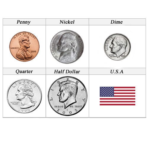
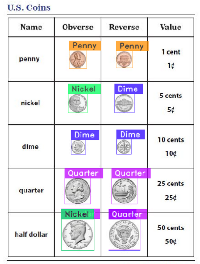
Note, we didn’t have a class for the half-dollar coin. So it will likely get classified as something else.
img_url = 'https://www.mynumi.net/media/catalog/product/cache/2/image/9df78eab33525d08d6e5fb8d27136e95/s/e/serietta_usa_2_1/www.mynumi.net-USASE5AD160-31.jpg'
best_model.predict(img_url).show()
The results aren’t too bad after just a few epochs!
References
↪️ 🏎️YOLO-NAS Starter Notebook

