Estimating Uncertainty in Machine Learning Models — Part 3
In the last part of our series on uncertainty estimation, we addressed the limitations of approaches like bootstrapping for large models, and demonstrated how we might estimate uncertainty in the predictions of a neural network using MC Dropout.
So far, the approaches we have looked at have involved creating variations in the dataset, or the model parameters to estimate uncertainty. The main drawback here is that it requires us to either train multiple models, or make multiple predictions in order to figure out the variance in our model’s predictions.
In situations with latency constraints, techniques such as MC Dropout might not be appropriate for estimating a prediction interval. What can we do to reduce the number of predictions we need to estimate the interval?
Using Maximum Likelihood Method (MLE) to estimate Intervals
In part 1 of this series, we made an assumption that the mean response of our dependent variable, μ(y|x),is normally distributed.
The MLE method involves building two models, one to estimate the conditional mean response, μ(y|x) , and another to estimate the variance, σ² in the predicted response.
We do this by first, splitting our training data into two halves. The first half model, mμ is trained as a regular regression model, using the first half of the data. This model is then used to make predictions on the second half of the data.
The second model, mσ² is trained using the second half of the data, and the squared residuals of mμ as the dependent variable.


The final prediction interval can be expressed in the following way

Here α is the desired level of confidence according to the Gaussian Distribution.
Let’s try it out
We’re going to be using the Auto MPG dataset again. Notice how the training data is split again in the last step.
Mean Variance Estimation Method

dataset_path = keras.utils.get_file("auto-mpg.data", "http://archive.ics.uci.edu/ml/machine-learning-databases/auto-mpg/auto-mpg.data")
column_names = ['MPG','Cylinders','Displacement','Horsepower','Weight',
                'Acceleration', 'Model Year', 'Origin']
raw_dataset = pd.read_csv(dataset_path, names=column_names,
                      na_values = "?", comment='\t',
                      sep=" ", skipinitialspace=True)

dataset = raw_dataset.copy()
dataset = dataset.dropna()

origin = dataset.pop('Origin')

dataset['USA'] = (origin == 1)*1.0
dataset['Europe'] = (origin == 2)*1.0
dataset['Japan'] = (origin == 3)*1.0

train_dataset = dataset.sample(frac=0.8,random_state=0)
test_dataset = dataset.drop(train_dataset.index)

mean_dataset = train_dataset.sample(frac=0.5 , random_state=0)
var_dataset = train_dataset.drop(mean_dataset.index)
Next, we’re going to create two models to estimate the mean and variance in our data
import keras

from keras.models import Model
from keras.layers import Input, Dense, Dropout
dropout_rate = 0.5

def model_fn():
    inputs = Input(shape=(9,))
    x = Dense(64, activation='relu')(inputs)
    x = Dropout(dropout_rate)(x)
    x = Dense(64, activation='relu')(x)
    x = Dropout(dropout_rate)(x)
    outputs = Dense(1)(x)

    model = Model(inputs, outputs)

    return model

mean_model = model_fn()
mean_model.compile(loss="mean_squared_error", optimizer='adam')

var_model = model_fn()
var_model.compile(loss="mean_squared_error", optimizer='adam')
Finally, we’re going to normalize our data, and start training
train_stats = train_dataset.describe()
train_stats.pop("MPG")
train_stats.transpose()

def norm(x):
    return (x - train_stats.loc['mean']) / train_stats.loc['std']

normed_train_data = norm(train_dataset)
normed_mean_data = norm(mean_dataset)
normed_var_data = norm(var_dataset)
normed_test_data = norm(test_dataset)

train_labels = train_dataset.pop('MPG')
mean_labels = mean_dataset.pop('MPG')
var_labels = var_dataset.pop('MPG')
test_labels = test_dataset.pop('MPG')
Once the mean model has been trained, we can use it to make predictions on the second half of our dataset and compute the squared residuals.
EPOCHS = 100

mean_model.fit(normed_mean_data, mean_labels, epochs=EPOCHS, validation_split=0.2, verbose=0)

mean_predictions = mean_model.predict(normed_var_data)
squared_residuals = (var_labels.values.reshape(-1,1) - mean_predictions) ** 2

var_model.fit(normed_var_data, squared_residuals, epochs=EPOCHS, validation_split=0.2, verbose=0)
Let’s take a look at the intervals produced by this approach.
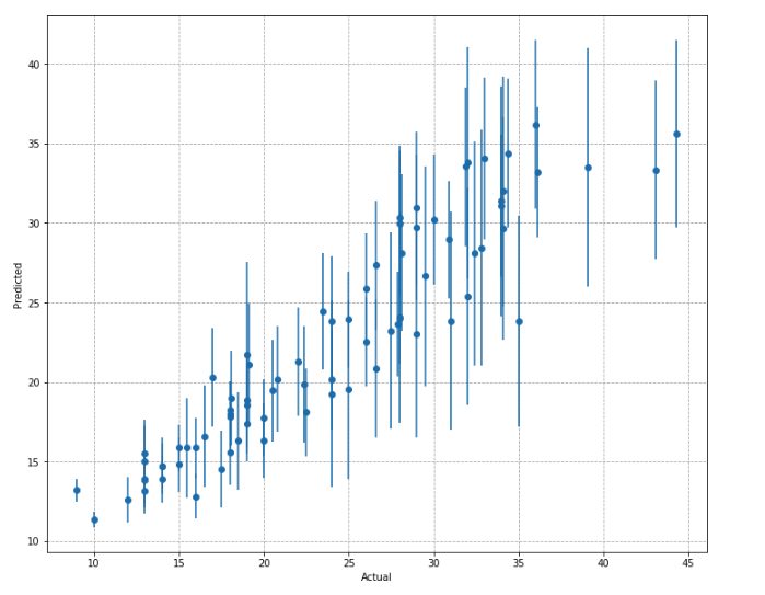
You will notice that the highly inaccurate predictions have much larger intervals around the mean.
Using Quantile Regression to Estimate Intervals
What if we do not want to make assumptions about the distribution of our response variable, and want to directly estimate the upper and lower limit of our target variable?
A quantile loss can help us estimate a target percentile response, instead of a mean response. i.e. Predicting the 0.25th Quantile value of our target will tell us, that given our current set of features, we expect 25% of the target values to be equal to, or less than our prediction.
If we train two separate regression models, one for the 0.025 percentile and another for the 0.9725 percentile, we are effectively saying that we expect 95% of our target values to fall within this interval i.e. A 95% prediction interval

Let’s try it out
Keras, does not come with a default quantile loss, so we’re going to use the following implementation from Sachin Abeywardana
import keras.backend as K

def tilted_loss(q,y,f):
    e = (y-f)
    return K.mean(K.maximum(q*e, (q-1)*e), axis=-1)

model = model_fn()
model.compile(loss=lambda y,f: tilted_loss(0.5,y,f), optimizer='adam')

lowerq_model = model_fn()
lowerq_model.compile(loss=lambda y,f: tilted_loss(0.025,y,f), optimizer='adam')

upperq_model = model_fn()
upperq_model.compile(loss=lambda y,f: tilted_loss(0.9725,y,f), optimizer='adam')
The resulting predictions look like this
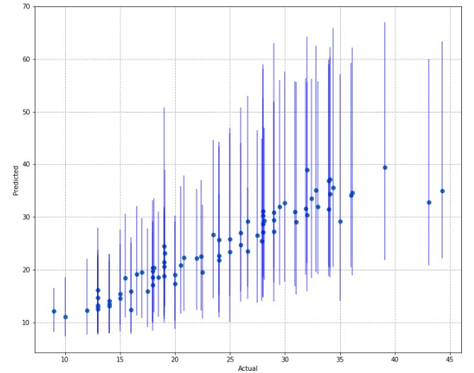
One of the disadvantages of this approach is that it tends to produce very wide intervals. You will also notice that the intervals are not symmetric about the median estimated values (blue dots).
Evaluating the Predicted Intervals
In the last post, we introduced two metrics to assess the quality of our interval predictions, PICP, and MPIW. The table below compares these metrics across the last three approaches we have used to estimate uncertainty in a Neural Network.
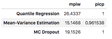
We see that the Mean-Variance estimation method produces the intervals with the smallest width, which results in a reduction of it’s PICP score. MC Dropout, and Quantile Regression produce very wide intervals, leading to a perfect PICP score.
Balancing between MPIW and PICP is an open ended question, and completely dependent on how the model is being applied. Ideally, we would like our intervals to be as tight as possible, with a low mean width, and also includes our target values the majority of time.
Conclusion
These techniques can readily be implemented on top of your existing models with very few changes, and providing uncertainty estimates to your predictions, makes them significantly more trustworthy.
I hope you enjoyed our series on uncertainty. Keep watching this space for more great content!!

