The 4 Advanced RAG Algorithms You Must Know to Implement
Welcome to Lesson 5 of 12 in our free course series, LLM Twin: Building Your Production-Ready AI Replica. You’ll learn how to use LLMs, vector DVs, and LLMOps best practices to design, train, and deploy a production ready “LLM twin” of yourself. This AI character will write like you, incorporating your style, personality, and voice into an LLM. For a full overview of course objectives and prerequisites, start with Lesson 1.
Lessons
- An End-to-End Framework for Production-Ready LLM Systems by Building Your LLM Twin
- Your Content is Gold: I Turned 3 Years of Blog Posts into an LLM Training
- I Replaced 1000 Lines of Polling Code with 50 Lines of CDC Magic
- SOTA Python Streaming Pipelines for Fine-tuning LLMs and RAG — in Real-Time!
- The 4 Advanced RAG Algorithms You Must Know to Implement
- Turning Raw Data Into Fine-Tuning Datasets
- 8B Parameters, 1 GPU, No Problems: The Ultimate LLM Fine-tuning Pipeline
- The Engineer’s Framework for LLM & RAG Evaluation
- Beyond Proof of Concept: Building RAG Systems That Scale
- The Ultimate Prompt Monitoring Pipeline
- [Bonus] Build a scalable RAG ingestion pipeline using 74.3% less code
- [Bonus] Build Multi-Index Advanced RAG Apps
In Lesson 5, we will focus on building an advanced retrieval module used for RAG.
We will show you how to implement 4 retrieval and post-retrieval advanced optimization techniques to improve the accuracy of your RAG retrieval step.
In this lesson, we will focus only on the retrieval part of the RAG system.
In Lesson 4, we showed you how to clean, chunk, embed, and load social media data to a Qdrant vector DB (the ingestion part of RAG).
In future lessons, we will integrate this retrieval module into the inference pipeline for a full-fledged RAG system.
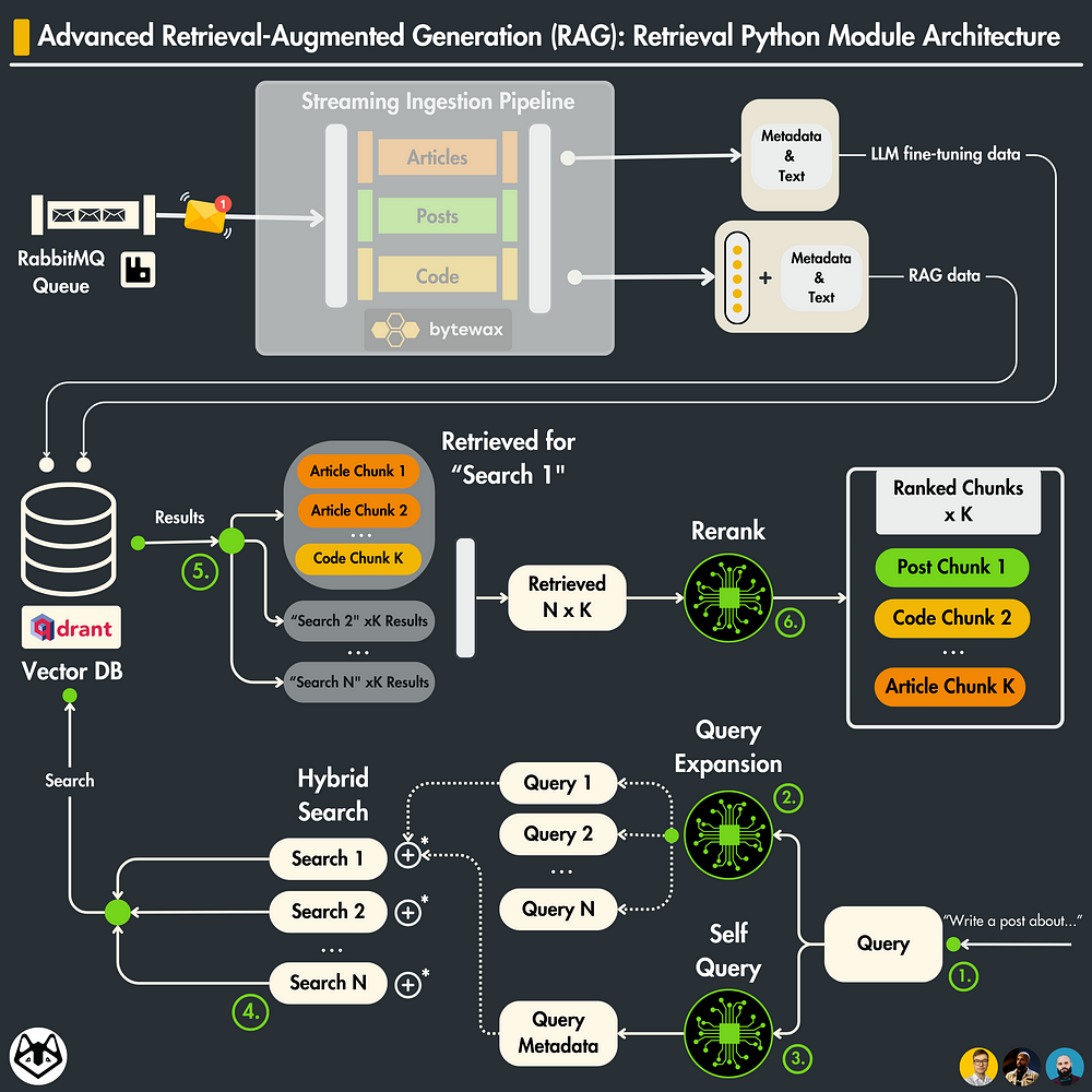
We assume you are already familiar with what a naive RAG looks like. If not, check out this article from Decoding ML.
Table of Contents
- Overview of advanced RAG optimization techniques
- Advanced RAG techniques applied to the LLM twin
- Retrieval optimization (1): Query expansion
- Retrieval optimization (2): Self query
- Retrieval optimization (3): Hybrid & filtered vector search
- Implement the advanced retrieval Python class
- Post-retrieval optimization: Rerank using GPT-4
- Running the RAG retrieval module
🔗 Check out the code on GitHub [1] and support us with a ⭐️
1. Overview of advanced RAG optimization techniques
A production RAG system is split into 3 main components:
- Ingestion: clean, chunk, embed, and load your data to a vector DB
- Retrieval: query your vector DB for context
- Generation: attach the retrieved context to your prompt and pass it to an LLM
The ingestion component sits in the feature pipeline, while the retrieval and generation components are implemented inside the inference pipeline.
You can also use the retrieval and generation components in your training pipeline to fine-tune your LLM further on domain-specific prompts.
You can apply advanced techniques to optimize your RAG system for ingestion, retrieval and generation.
That being said, there are 3 main types of advanced RAG techniques:
- Pre-retrieval optimization [ingestion]: tweak how you create the chunks
- Retrieval optimization [retrieval]: improve the queries to your vector DB
- Post-retrieval optimization [retrieval]: process the retrieved chunks to filter out the noise
The generation step can be improved through fine-tuning or prompt engineering, which will be explained in future lessons.
The pre-retrieval optimization techniques are explained in Lesson 4.
In this lesson, we will show you some popular retrieval and post-retrieval optimization techniques.
2. Advanced RAG techniques applied to the LLM twin
Retrieval optimization
We will combine 3 techniques:
- Query Expansion
- Self Query
- Filtered vector search
Post-retrieval optimization
We will use the rerank pattern using GPT-4 and prompt engineering instead of Cohere or an open-source re-ranker cross-encoder [4].
I don’t want to spend too much time on the theoretical aspects. There are plenty of articles on that.
So, we will jump straight to implementing and integrating these techniques in our LLM twin system.
But before seeing the code, let’s clarify a few things ↓

2.1 Important Note!
We will show you a custom implementation of the advanced techniques and NOT use LangChain.
Our primary goal is to build your intuition about how they work behind the scenes. However, we will attach LangChain’s equivalent so you can use them in your apps.
Customizing LangChain can be a real headache. Thus, understanding what happens behind its utilities can help you build real-world applications.
Also, it is critical to know that if you don’t ingest the data using LangChain, you cannot use their retrievals either, as they expect the data to be in a specific format.
We haven’t used LangChain’s ingestion function in Lesson 4 either (the feature pipeline that loads data to Qdrant) as we want to do everything “by hand”.
2.2. Why Qdrant?
There are many vector DBs out there, too many…
But since we discovered Qdrant, we loved it.
Why?
- It is built in Rust.
- Apache-2.0 license — open-source 🔥
- It has a great and intuitive Python SDK.
- It has a freemium self-hosted version to build PoCs for free.
- It supports unlimited document sizes, and vector dims of up to 645536.
- It is production-ready. Companies such as Disney, Mozilla, and Microsoft already use it.
- It is one of the most popular vector DBs out there.
To put that in perspective, Pinecone, one of its biggest competitors, supports only documents with up to 40k tokens and vectors with up to 20k dimensions…. and a proprietary license.
I could go on and on…
…but if you are curious to find out more, check out Qdrant ←
3. Retrieval optimization (1): Query expansion
The problem
In a typical retrieval step, you query your vector DB using a single point.
The issue with that approach is that by using a single vector, you cover only a small area of your embedding space.
Thus, if your embedding doesn’t contain all the required information, your retrieved context will not be relevant.
What if we could query the vector DB with multiple data points that are semantically related?
That is what the “Query expansion” technique is doing!
The solution
Query expansion is quite intuitive.
You use an LLM to generate multiple queries based on your initial query.
These queries should contain multiple perspectives of the initial query.
Thus, when embedded, they hit different areas of your embedding space that are still relevant to our initial question.
You can do query expansion with a detailed zero-shot prompt.
Here is our simple & custom solution ↓
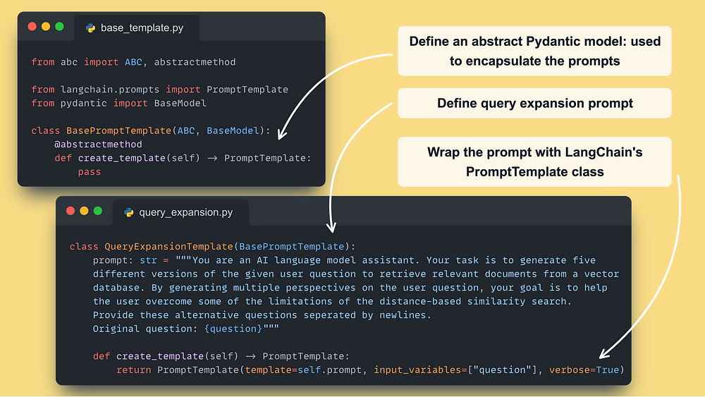
Here is LangChain’s MultiQueryRetriever class [5] (their equivalent).
4. Retrieval optimization (2): Self query
The problem
When embedding your query, you cannot guarantee that all the aspects required by your use case are present in the embedding vector.
For example, you want to be 100% sure that your retrieval relies on the tags provided in the query.
The issue is that by embedding the query prompt, you can never be sure that the tags are represented in the embedding vector or have enough signal when computing the distance against other vectors.
The solution
What if you could extract the tags within the query and use them along the embedded query?
That is what self-query is all about!
You use an LLM to extract various metadata fields that are critical for your business use case (e.g., tags, author ID, number of comments, likes, shares, etc.)
In our custom solution, we are extracting just the author ID. Thus, a zero-shot prompt engineering technique will do the job.
But, when extracting multiple metadata types, you should also use few-shot learning to optimize the extraction step.
Self-queries work hand-in-hand with vector filter searches, which we will explain in the next section.
Here is our solution ↓
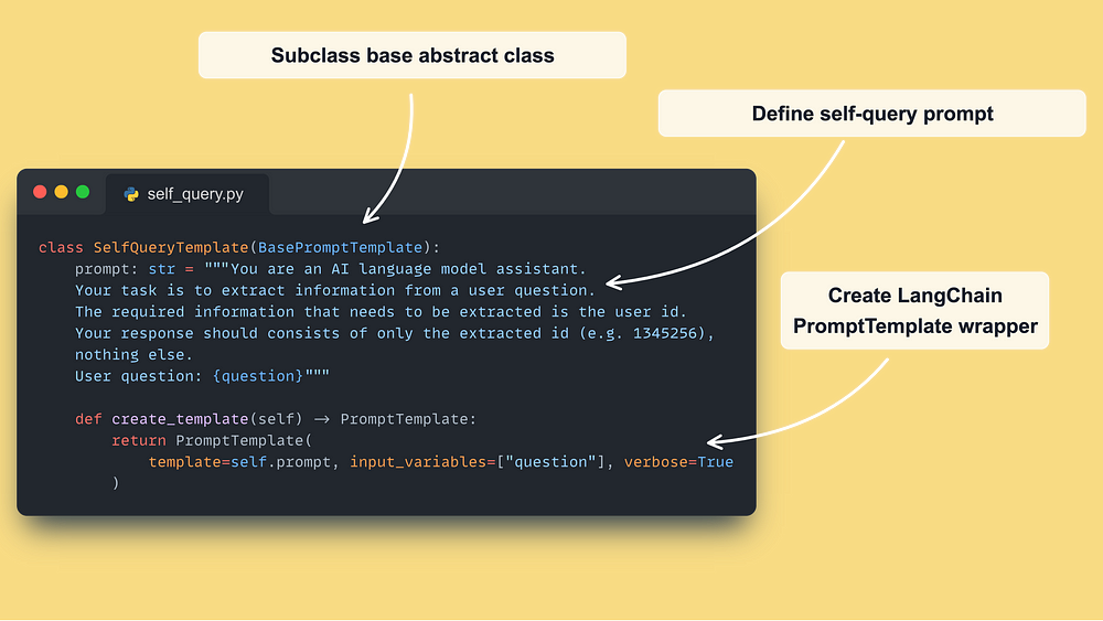
Here is LangChain’s SelfQueryRetriever class [6] equivalent and this is an example using Qdrant [8].
5. Retrieval optimization (3): Hybrid & filtered vector search
The problem
Embeddings are great for capturing the general semantics of a specific chunk.
But they are not that great for querying specific keywords.
For example, if we want to retrieve article chunks about LLMs from our Qdrant vector DB, embeddings would be enough.
However, if we want to query for a specific LLM type (e.g., LLama 3), using only similarities between embeddings won’t be enough.
Thus, embeddings are not great for finding exact phrase matching for specific terms.
The solution
Combine the vector search technique with one (or more) complementary search strategy, which works great for finding exact words.
It is not defined which algorithms are combined, but the most standard strategy for hybrid search is to combine the traditional keyword-based search and modern vector search.
How are these combined?
The first method is to merge the similarity scores of the 2 techniques as follows:
hybrid_score = (1 - alpha) * sparse_score + alpha * dense_score Where alpha takes a value between [0, 1], with:
- alpha = 1: Vector Search
- alpha = 0: Keyword search
Also, the similarity scores are defined as follows:
- sparse_score: is the result of the keyword search that, behind the scenes, uses a BM25 algorithm [7] that sits on top of TF-IDF.
- dense_score: is the result of the vector search that most commonly uses a similarity metric such as cosine distance
The second method uses the vector search technique as usual and applies a filter based on your keywords on top of the metadata of retrieved results.
→ This is also known as filtered vector search.
In this use case, the similar score is not changed based on the provided keywords.
It is just a fancy word for a simple filter applied to the metadata of your vectors.
But it is essential to understand the difference between the first and second methods:
- The first method combines the similarity score between the keywords and vectors using the alpha parameter;
- The second method is a simple filter on top of your vector search.
How does this fit into our architecture?
Remember that during the self-query step, we extracted the author_id as an exact field that we have to match.
Thus, we will search for the author_id using the keyword search algorithm and attach it to the 5 queries generated by the query expansion step.
As we want the most relevant chunks from a given author, it makes the most sense to use a filter using the author_id as follows (filtered vector search) ↓
 self._qdrant_client.search(
      collection_name="vector_posts",
      query_filter=models.Filter(
          must=[
              models.FieldCondition(
                  key="author_id",
                  match=models.MatchValue(
                      value=metadata_filter_value,
                  ),
              )
          ]
      ),
      query_vector=self._embedder.encode(generated_query).tolist(),
      limit=k,
)
Note that we can easily extend this with multiple keywords (e.g., tags), making the combination of self-query and hybrid search a powerful retrieval duo.
The only question you have to ask yourself is whether we want to use a simple vector search filter or the more complex hybrid search strategy.
Note that LangChain’s SelfQueryRetriever class combines the self-query and hybrid search techniques behind the scenes, as can be seen in their Qdrant example [8]. That is why we wanted to build everything from scratch.
6. Implement the advanced retrieval Python class
Now that you’ve understood the advanced retrieval optimization techniques we’re using, let’s combine them into a Python retrieval class.
Here is what the main retriever function looks like ↓
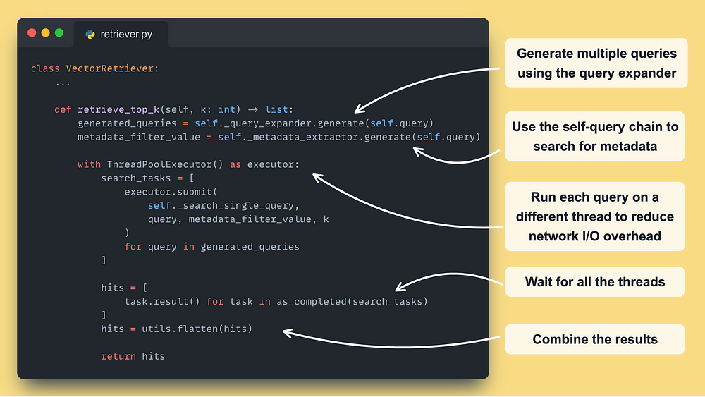
Using a Python ThreadPoolExecutor is extremely powerful for addressing I/O bottlenecks, as these types of operations are not blocked by Python’s GIL limitations.
Here is how we wrapped every advanced retrieval step into its own class ↓
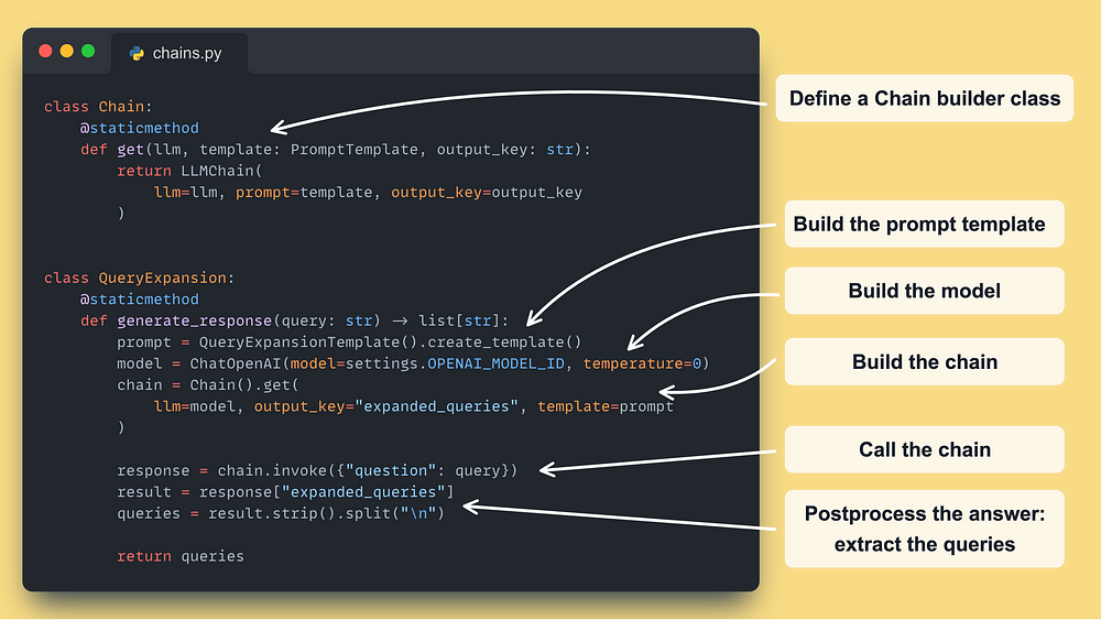
The SelfQuery class looks very similar — 🔗 access it here [1] ←.
The final step is to call Qdrant for each query generated by the query expansion step ↓
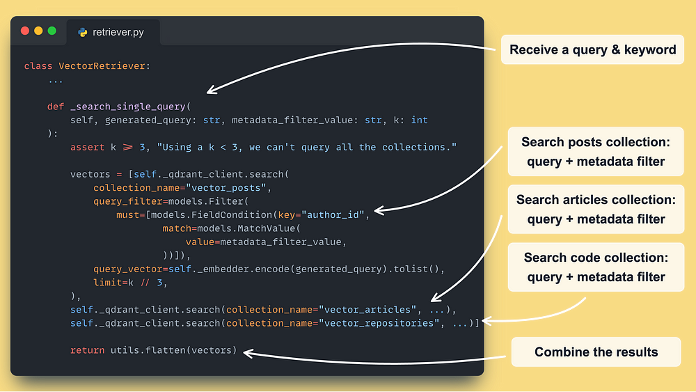
Note that we have 3 types of data: posts, articles, and code repositories.
Thus, we have to make a query for each collection and combine the results in the end.
The most performant method is to use multi-indexing techniques, which allow you to query multiple types of data at once.
But at the time I am writing this article, this is not a solved problem at the production level.
Thus, we gathered data from each collection individually and kept the best-retrieved results using rerank.
Which is the final step of the article.
7. Post-retrieval optimization: Rerank using GPT-4
We made a different search in the Qdrant vector DB for N prompts generated by the query expansion step.
Each search returns K results.
Thus, we end up with N x K chunks.
In our particular case, N = 5 & K = 3. Thus, we end up with 15 chunks.
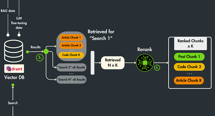
The problem
The retrieved context may contain irrelevant chunks that only:
- Add noise: the retrieved context might be irrelevant
- Make the prompt bigger: results in higher costs & the LLM is usually biased in looking only at the first and last pieces of context. Thus, if you add a big context, there is a big chance it will miss the essence.
- Unaligned with your question: the chunks are retrieved based on the query and chunk embedding similarity. The issue is that the embedding model is not tuned to your particular question, which might result in high similarity scores that are not 100% relevant to your question.
The solution
We will use rerank to order all the N x K chunks based on their relevance relative to the initial question, where the first one will be the most relevant and the last chunk the least.
Ultimately, we will pick the TOP K most relevant chunks.
Rerank works really well when combined with query expansion.
A natural flow when using rerank is as follows:
Search for >K chunks >>> Reorder using rerank >>> Take top K
Thus, when combined with query expansion, we gather potential useful context from multiple points in space rather than just looking for more than K samples in a single location.
Now the flow looks like:
Search for N x K chunks >>> Reoder using rerank >>> Take top K
A typical solution for reranking is to use open-source Bi-Encoders from sentence transformers [4].
These solutions take both the question and context as input and return a score from 0 to 1.
In this article, we want to take a different approach and use GPT-4 + prompt engineering as our reranker.
If you want to see how to apply rerank using open-source algorithms, check out this hands-on article from Decoding ML.
Now let’s see our implementation using GPT-4 & prompt engineering.
Similar to what we did for the expansion and self-query chains, we define a template and a chain builder ↓
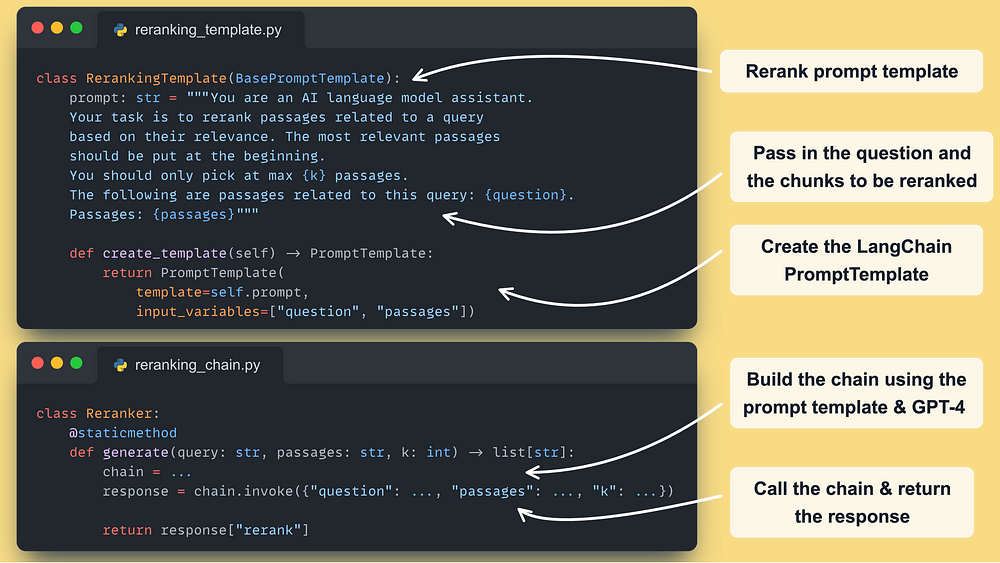
Here is how we integrate the rerank chain into the retriever:
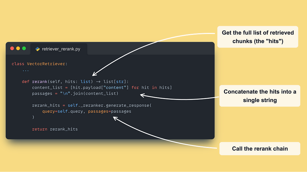
…and that’s it!
Note that this is an experimental process. Thus, you can further tune your prompts for better results, but the primary idea is the same.
→ Find the complete code used in this lesson in our GitHub at core/rag
8. Running the RAG retrieval module
The last step is to run the whole thing.
But there is a catch.
As initially said, the retriever will not be used as a standalone component in the LLM system.
The inference pipeline will use it as a layer between the data and the Qdrant vector DB to do RAG.
Still, to check that everything works fine, let’s test out the RAG retrieval module as a standalone script.
We can call the VectorRetriever module using the following code as an example:
 from core import get_logger
from core.config import settings
from core.rag.retriever import VectorRetriever

logger = get_logger(__name__)


query = """
Hello I am Paul Iusztin.

Could you draft an article paragraph discussing RAG?
I'm particularly interested in how to design a RAG system.
"""

  retriever = VectorRetriever(query=query)
  hits = retriever.retrieve_top_k(k=6, to_expand_to_n_queries=5)
  reranked_hits = retriever.rerank(hits=hits, keep_top_k=5)

  logger.info("====== RETRIEVED DOCUMENTS ======")
  for rank, hit in enumerate(reranked_hits):
      logger.info(f"Rank = {rank} : {hit}")
To spin up locally the Qdrant vector DB in a Docker container, run:
make local-start To populate it with data, run the following:
make local-ingest-dataNow, to test out the script from above, run:
make local-test-retrieverIt should print the most similar hits found in the Qdrant vector DB to the CLI.
…and that’s it!
In future lessons, we will learn to integrate it into the inference pipeline for an end-to-end RAG system.
Conclusion
In Lesson 5, you learned to build an advanced RAG retrieval module optimized for searching posts, articles, and code repositories from a Qdrant vector DB.
First, you learned about where the RAG pipeline can be optimized:
- pre-retrieval
- retrieval
- post-retrieval
After you learn how to build from scratch (without using LangChain’s utilities) the following advanced RAG retrieval & post-retrieval optimization techniques:
- query expansion
- self query
- hybrid search
- rerank
Ultimately, you understood where the retrieval component sits in an RAG production LLM system, where the code is shared between multiple microservices and doesn’t sit in a single Notebook.
In Lesson 6, we will move to the training pipeline and show you how to automatically transform the data crawled from LinkedIn, Substack, Medium, and GitHub into an instruction dataset using GPT-4 to fine-tune your LLM Twin.
See you there! 🤗
🔗 Check out the code on GitHub [1] and support us with a ⭐️
References
Literature
[1] Your LLM Twin Course — GitHub Repository (2024), Decoding ML GitHub Organization
[2] Bytewax, Bytewax Landing Page
[3] Qdrant, Qdrant Documentation
[4] Retrieve & Re-Rank, Sentence Transformers Documentation
[5] MultiQueryRetriever, LangChain’s Documentation
[6] Self-querying, LangChain’s Documentation
[7] Okapi BM25, Wikipedia
[8] Qdrant Self Query Example, LangChain’s Documentation
Images
If not otherwise stated, all images are created by the author.

