4 Techniques To Tackle Overfitting In Deep Neural Networks
 Image Created By Author Using Canva
A neural network is a combination of different neurons, layers, weights, and biases. The first neural network was created in 1957 and named perceptron. It is similar to modern-day neural networks but it only had one layer. Since then, neural networks have become widely used for making predictions and business decisions.
Neural networks became famous because of their ability to beat any traditional machine learning algorithm by a long margin in terms of performance. After the first neural network, they have evolved so much that nowadays there are networks with tons of layers and billions of parameters.
With the involvement of APIs like Keras, Tensorflow, and Pytorch it has become very easy to design a neural network to achieve good accuracy on any kind and size of data. Being so powerful in terms of architecture, neural networks, if not created properly, can fall into the problem of overfitting.
Overfitting is a condition that occurs when a model performs significantly better for training data than it does for new data. In this blog, we will see some of the techniques that are helpful for tackling overfitting in neural networks.
Data Augmentation
The simplest way to eliminate overfitting is data augmentation. Data augmentation is the process of reproducing new training instances from existing ones. It is commonly used in computer vision to regenerate images for convolutional neural networks.
Image augmentation is a type of data augmentation technique in which we apply certain transformations to our images to produce multiple copies of the original image that are totally different in terms of size and colors from the original image.
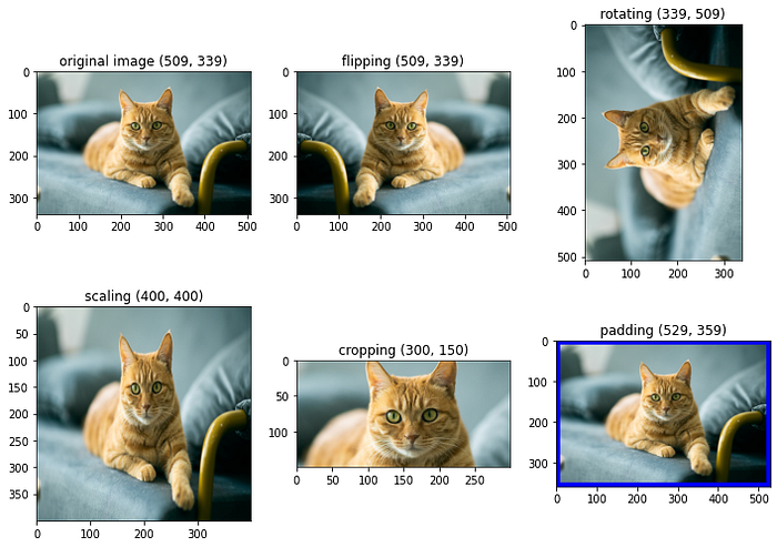
Position and Color are the two most common transformation techniques that are used to reproduce data. Position augmentation changes the pixel position of an image. Some famous techniques to do so are — scaling, cropping, flipping, padding, rotation, and translation at different positional values.
from PIL import Image
import matplotlib.pyplot as pltimg = Image.open("/content/drive/MyDrive/cat.jpg")
flipped_img = img.transpose(Image.FLIP_LEFT_RIGHT) ###flipping
roated_img = img.transpose(Image.ROTATE_90) ## rotating
scaled_img = img.resize((400, 400))  ### scaling##left, upper, right, lower
cropped_img = img.crop((100,50,400,200))width, height = img.size
pad_pixel = 20
canvas = Image.new(img.mode, (width+pad_pixel, height+pad_pixel), 'blue')
canvas.paste(img, (pad_pixel//2,pad_pixel//2))
 Position Augmentation
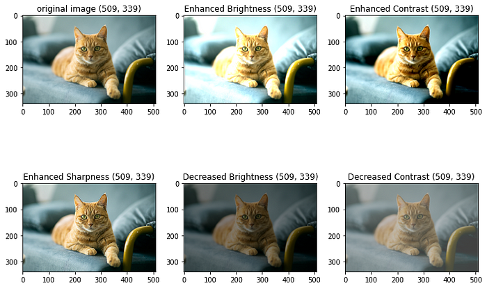
Color Augmentation deals with altering the color properties of an image by changing its pixel values. Some of the most common techniques of it are changing brightness, contrast, saturation, hue, grayscale, dilation, etc.
from PIL import Image, ImageEnhance
import matplotlib.pyplot as plt
img = Image.open("/content/drive/MyDrive/cat.jpg")enhancer = ImageEnhance.Brightness(img)
img2 = enhancer.enhance(1.5)  ## brightens image
img3 = enhancer.enhance(0.5)  ## darkens imageenhancer = ImageEnhance.Contrast(img)
img4 = enhancer.enhance(1.5) ## increase contrast
img5 = enhancer.enhance(0.5) ## decrease contrastenhancer = ImageEnhance.Sharpness(img)
img6 = enhancer.enhance(5) ## increase sharpness

Although it is possible to perform image augmentation manually by using image processing libraries like pillow and OpenCV, the much simpler and less time-consuming way is to do it by using the Keras API.
Keras is a deep learning API written in Python, running on top of the machine learning platform Tensorflow. Keras has many inbuild methods and classes that increase the experimentation speed. In Keras, inside the image class, we have a method ImageDataGenerator that provides multiple options for Image Augmentation.
keras.preprocessing.image.ImageDataGenerator()
arguments:
1. featurewise_center: Truth value. Average the inputs to 0 for the entire dataset.
2. samplewise_center: Truth value. Set the average of each sample to 0.
3. featurewise_std_normalization: Truth value. Normalizes the input with the standard deviation of the dataset.
4. samplewise_std_normalization: Truth value. Normalize each input with its standard deviation.
5. zca_epsilon: ZCA whitening epsilon. The default is 1e-6.
6. zca_whitening: Truth value. Apply ZCA whitening.
7. rotation_range: Integer. A rotation range that randomly rotates the image.
8. width_shift_range: Floating point number (ratio to width). Random horizontal shift range.
9. height_shift_range: Floating point number (ratio to vertical width). Random vertical shift range.
10. shear_range: Floating point number. Shear strength (counterclockwise shear angle).
11. zoom_range: Floating point number or [lower, upper]. Random zoom range. Given a floating point number [lower, upper] = [1-zoom_range, 1+zoom_range]:
12. channel_shift_range: Floating point number. The range in which the channel is randomly shifted.
13. horizontal_flip: Truth value. Randomly inverts the input horizontally.
14. vertical_flip: Truth value. Randomly inverts the input in the vertical direction.
15. rescale: Pixel value rescale factor. The default is None. If None or 0, it does not apply.
16. preprocessing_function: Function applied to each input. This function will be executed before any other changes are made.
17. validation_split: Floating point number. Percentage of images reserved for verification (strictly between 0 and 1).
18. fill_mode: {“constant”, “nearest”, “reflect”, “wrap”} The default is ‘nearest’. Fills around the boundaries of the input image according to the specified mode.
19. cval: Floating point number or integer. fill_mode = "constant"The value used around the boundary at.
Performing Data Augmentation using Tensorflow
from keras.preprocessing.image import ImageDataGenerator, array_to_img, img_to_array, load_img

datagen = ImageDataGenerator(
        rotation_range=40,
        width_shift_range=0.2,
        height_shift_range=0.2,
        brightness_range= [0.5, 1.5],
        rescale=1./255,
        shear_range=0.2,
        zoom_range=0.4,
        horizontal_flip=True,
        fill_mode='nearest',
        zca_epsilon=True)

path = '/content/drive/MyDrive/cat.jpg' ## Image Path
img = load_img(f"{path}")
x = img_to_array(img)
x = x.reshape((1,) + x.shape)
i = 0

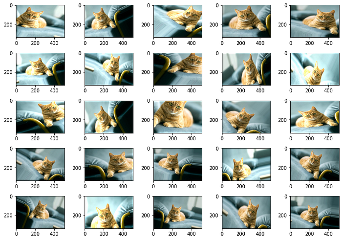
### Create 25 Augmentated Images and Save Them In `aug_img` directory
for batch in datagen.flow(x, batch_size=1,
                      save_to_dir="/content/drive/MyDrive/aug_imgs", save_prefix='img', save_format='jpeg'):
    i += 1
    if i > 25:   ## Total 25 Augmented Images
        break

There are many advanced methods as well that make use of Generative Adversarial Networks (GANs) to perform data augmentation. You can read about these methods by reading these research papers:
1. Data augmentation using Generative Adversarial Networks (GANs) for GAN-based detection of Pneumonia and COVID-19 in chest X-ray images
2. Data Augmentation Generative Adversarial Networks
Adding Dropout Layers
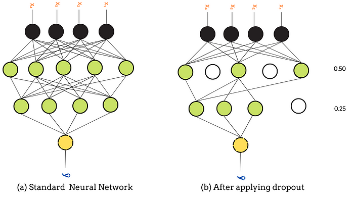
Dropout layers are the most common method to tackle overfitting in deep neural networks. It reduces the chances of overfitting by modifying the network.
Dropout layers randomly set input units to 0 with a frequency of rate at each step during the training phase. These inputs with 0 frequency are dropped for the same training epoch. Inputs not set to 0 are scaled up by 1/(1 — rate) such that the sum over all inputs is unchanged.
Rate is the main parameter that ranges from 0 to 1. It specifies the fraction of the input units to drop. For example, the rate of 0.5 means 50% of units (neurons) are dropped randomly from the network.

tf.keras.layers..Dropout(rate, noise_shape=None, seed=None)
arguments
1. rate : Float between 0 and 1. Fraction of the input units to drop.
2. noise_shape :1D integer tensor representing the shape of the binary dropout mask that will be multiplied with the input.
3. seed : Integer to use as a random seed.
Adding Dropout Layers Using Tensorflow
import tensorflow as tf
from tensorflow.keras.models import Sequential
from tensorflow.keras.layers import Dense,Reshape
from tensorflow.keras.layers import Dropout

def create_model():
  model = Sequential()
  model.add(Dense(60, input_shape=(60,), activation='relu'))
  model.add(Dropout(0.2))
  model.add(Dense(30, activation='relu'))
  model.add(Dropout(0.2))
  model.add(Dense(1, activation='sigmoid'))
  return model

adam = tf.keras.optimizers.Adam()
model.compile(loss='binary_crossentropy', optimizer=adam, metrics=['accuracy'])

model = create_model()
model.summary()

There are certain tips that you should consider while adding dropout layers to your neural network:
1. Use a small dropout value of 20%-50% of neurons. Specifying a larger dropout value might decrease the model performance also choosing a very small value will not affect the network much.
2. Try to dropout layer only in a large network to get maximum performance.
3. You can use dropout on incoming (visible) and hidden layers both. It performs well in both cases.
Want to get the most up-to-date news on all things Deep Learning? Subscribe to Deep Learning Weekly for the latest research, resources, and industry news, delivered to your inbox.
L1 and L2 Regularization
Regularization is a technique to reduce the complexity of the network by penalizing the loss function. It adds an extra element to the loss function, which punishes our model for being too complex or, in simple words, for using high values in the weight matrix.
L1 Regularization reduces the weight values for less important features to zero so that only important features take part in the training and validation process. It works as an automatic feature selector for neural networks. It is also referred to as Least Absolute Deviations, and minimizes the absolute difference between target and estimated(predicted) values.

L2 Regularization forces the weights towards zero but never makes them exactly zero. It removes a small percentage of weight at each iteration to reduce the complexity of the network and make it simple so that it does not overfit on the data. It minimizes the square of the sum of the difference between target values and estimated values.

Performing Regularization Using Tensorflow
import tensorflow as tf
from tensorflow.keras.models import Sequential
from tensorflow.keras.layers import Dense,Reshape
from tensorflow.keras.layers import Dropout

def create_model():
  # create model
  model = Sequential()
  model.add(Dense(60, input_shape=(60,), activation='relu',  kernel_regularizer=keras.regularizers.l1(0.01)))
  model.add(Dropout(0.2))
  model.add(Dense(30, activation='relu',  kernel_regularizer=keras.regularizers.l2(0.001)))
  model.add(Dropout(0.2))
  model.add(Dense(1, activation='sigmoid'))
  return model


adam = tf.keras.optimizers.Adam()
model.compile(loss='binary_crossentropy', optimizer=adam, metrics=['accuracy'])

model = create_model()
model.summary()
You can learn about L1 and L2 Regularization more deeply by reading the below research papers:
1. Feature selection, L1 vs. L2 regularization, and rotational invariance
2. Regularization Methods in Neural Networks
3. A Comparison of Regularization Techniques in Deep Neural Networks
Early Stopping
One epoch is one complete pass of training data through the neural network. During each epoch, each neuron has the opportunity to update its weights, so the more epochs you choose, the longer your training will be. Additionally, choosing too many epochs can lead to overfitting. On the other hand, choosing too few epochs can cause underfitting.
Early stopping is a form of regularization that stops the training process once model performance stops improving on the validation set as it significantly decreases the likelihood of overfitting the model.
Keras has a callback function designed to stop training early once it has detected that the model is no longer making significant improvements.
from tensorflow.keras.callbacks import EarlyStopping
early_stopping = EarlyStopping(
    monitor='val_loss',
    min_delta=0,
    patience=0,
    verbose=0,
    mode='auto',
    baseline=None,
    restore_best_weights=False
)
Arguments
monitor: metric to be used as a measure for terminating the training.
min_delta: change in the monitored quantity to qualify as an improvement. less min_delta will count as no improvement.
patience: number of epochs with no improvement after which training gets terminated.
verbose: Verbosity mode, 0 or 1. Mode 0 is silent, and mode 1 displays callback messages.
mode:{“auto”, “min”, “max”}, in minmode training, will stop when performance stops decreasing, in max mode training will stop when performance stops increasing, in "auto" mode, the direction is automatically inferred from the name of the monitored quantity.
baseline: baseline value for the monitored quality.
restore_best_weights: Whether to restore model weights from the epoch with the best value of the monitored quantity or not.
from tensorflow.keras.callbacks import EarlyStoppingearly_stopping = EarlyStopping(monitor='loss', patience=2)history = model.fit(
    X_train,
    y_train,
    epochs= 100,
    validation_split= 0.20,
    batch_size= 50,
    verbose= "auto",
    callbacks= [early_stopping]
)

Early stopping will stop the neural network when it stops improving for the specified number of epochs, thus reducing the training time taken by the network.
These methods only work when you apply them correctly. Not every network requires each technique to be applied, some networks can be improved by applying just one method.
Conclusion
As a quick recap of different techniques, data augmentation will increase the size of data by applying different transformations to images and dropout layers will reduce the network complexity by randomly dropping some neurons. Regularization techniques will penalize the network for producing large errors and, at the end, early stopping methods will stop the training of the network once it stops improving.


